
10 Incremental Investments
Lindon Robison
Learning goals. After completing this chapter, you should be able to: (1) distinguish between incremental and stand-alone investments; (2) understand how time and use costs determine the optimal service extraction rate from investments; and (3) find earnings and rates of return on incremental investments.
Learning objectives. To achieve your learning goals, you should complete the following objectives:
- Learn how to distinguish between incremental and stand-alone investments.
- Learn how an investment’s liquidation and acquisition values determine its fixity.
- Learn how an investment’s time and use costs determine its optimal service extraction rates.
- Learn how to find contributions from incremental investments by finding changes in the firm’s cash receipts (CR), cash cost of goods sold (COGS), cash overhead expenses (OE), and change in operating and capital asset accounts.
- Learn how to use Excel templates to find net present value (NPV), annuity equivalent (AE), and internal rate of return (IRR) measures earned by incremental investments.
Introduction
Think of two kinds of investments. The first one is a stand-alone investment—possibly including other supporting capital investments and nondurable inputs. The second kind of investment is an incremental one. We consider incremental investments when we want to add to or replace an investment that is part of an existing production unit. Firms that extract services from durables, especially those that depreciate, must some time replace or refurbish them, and the decision depends on what happens to the difference in NPV of the firm’s cash flow before and after the incremental investment.
Whether we invest in an incremental investment or disinvest in an existing investment depends on its asset’s fixity. A fixed investment is one already owned by the firm and unlikely to be removed from service. Glenn Johnson described the conditions required for an investment to be fixed; namely, that the investment’s acquisition value (V0) and liquidation value (V0liquidation) bound its value in use (V0use). In other words, an investment is fixed or unlikely to be removed from service if: V0liquidation < V0use < V0. Because the investment’s value in use is less than what it would cost to acquire another one and because its liquidation value is less than what it is earning—the firm has no incentive to invest or disinvest in them. An investment with a zero or negative liquidation value is one likely fixed if it contributes something positive to the firm.
We summarize the collective contributions of the firm’s capital assets during a single period as earnings in an accrual income statement (AIS). Then we calculate AIS earning as a percentage of the firm’s beginning assets and equity and report the results as return on assets (ROA) and returns on equity (ROE) measures.
AIS earnings estimates make no effort to find the contributions of a single capital asset or subset of the firm’s assets. However, isolating earnings from a single capital asset and possibly its supporting assets is exactly what we do when constructing PV models for firm investments—we attempt to isolate the return from the investment(s) added to the production unit or the firm. Otherwise, how can we decide to invest or not in the challenger?
However, we face a difficulty when we attempt to measure the returns from an incremental investment. The difficulty is that the firm’s optimal response to a new investment is often to change the levels of nondurable assets and services extracted from other durables operated by the firm making it difficult to identify what part of the output change we can attribute to the new investment versus output changes that should be attributed to changes in the use of other inputs employed by the firm. This problem, measuring the contributions of incremental investments will occupy much of our attention in this chapter.
What follows. In what the follows, we describe how to analyze incremental investments using incremental budgeting analysis. We introduce the incremental investment analysis using simplified mathematical methods and graphical analysis. Then we illustrate incremental budgeting analysis using Green & White Services example and this book’s generalized PV template described in Appendix to Chapter 8.
Measuring Contributions from Incremental Investments
An example of an incremental investment. To illustrate an incremental investment, suppose that Hi Quality Nursery (HQN) considers investing in a sprinkler system to reduce its demand for seasonal labor. HQN asks: will investing in the new sprinkler system improve my firm’s financial well-being?
How do we approach incremental investments differently compared to stand-alone investments? Or, in our example, how do we measure the financial consequences of the sprinkler investment and the reduction in hired labor? To find the answer: we find what changes in revenue and expenses will the sprinkler investment and the hired labor disinvestment produce for HQN?
We know that the new sprinkler system means that HQN can reduce its dependence on hourly workers to water its plants during the growing season. Furthermore, this change in HQN’s operating procedures will likely continue for many periods in the future. Some new expenses may be incurred associated with operating and maintaining the new sprinkler system, but these are likely to be much less than the reduction in hired labor resulting from the sprinkler investment. It’s not clear what changes in revenue would result from adopting a new watering system. It may be that a reduction in operating costs means that some unprofitable plants and shrubs may now be profitable because operating costs to produce them are less.
Because the consequences of the sprinkler/hired labor changes will likely have long-term consequences, this problem can’t be analyzed using a single period financial tool such as CFS. Instead the problem requires that we employ multi-period PV model templates. The answers that can be supplied by PV models include: how will an incremental investment change the capital structure of the firm? How will incremental investment change the equity of the firm? How will the incremental investment change the internal rate of return on the firm’s assets and equity?
Contributions from existing investments. Suppose that we have a profit function π that depends on the revenue and costs associated with an independent profit generating plant described as f(x) where the variable x represents the existing asset and liability configuration of the firm:
(10.1) 
Analyzing the firm as a function of its current asset and liability configuration described as x in equation (10.1) is what we do when we construct coordinated financial statements (CFS). Rates of return on assets and equity as well as our other ratio calculations all reflect the current financial condition of the firm. To find rates of return on assets or equity, we divide equation one by its assets or by its equity.
Now suppose that we want to analyze how profits will respond to a change in x. Using the delta notation, ∆ to reflect change, we write the effect of a change in x on profits as:
(10.2) 
What we have described is a stand-alone investment that allows us to examine the effects on profits in response to a change in x without being required to consider other changes in the firm. To complicate the analysis, suppose that the firm’s asset and liability configuration are describe by two interdependent variables x and y so that when we change x, to maximize profits we must also change y. Indeed, it is hard to imagine any change in x that doesn’t require adjustments in other inputs to achieve the most beneficial outcomes. (If we purchase a sprinkler to reduce labor costs, we would surely expect labor costs to be reduced). To account for the simultaneity of x and y, we write the profit function as:
(10.3) 
Since x and y are interdependent, any change in x must also consider a change y to optimize its firm profits, so that to analyze a change in profits attributable to a change in x and y, we must calculate:
(10.4) 
Equation (10.4) essentially describes incremental analysis. In accounts for changes in revenue and expenses associated with the incremental investments plus changes in the costs and revenue associated with other variables essential to the firm’s operations.
A graphical approach. We now present the earlier results using graphical analysis familiar to students of microeconomics. Assume that a firm produces output using a combination of capital services and other inputs x and y. We graph the combinations of capital services and other inputs that produce the same output and call the result an isoquant (i.e. same quantity). In Figure 10.1 we represent two levels of output by isoquants Q1, and Q2 drawn convex to the origin to reflect diminishing marginal productivity.
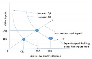
Now suppose that the firm considers an incremental investment, a capital investment that will allow the firm to increase its supply of capital services from CS1 to CS3 and increase output from Q1 to Q2. In this case, we hold constant the level of other inputs constant at OI1. However, economic production theory teaches that increasing production from Q1 to Q2 holding other inputs constant would be inefficient. Instead, the theory teaches that the firm should increase capital services and other inputs along some least cost line AC determined by the relative costs of increasing both the capital services from the new investment and from the other inputs.
Increasing production along the least cost line AC, the firm would increase capital service from CS1 to CS2 an amount less that was required to reach Q2 when we held other inputs constant. In other words, increasing the use of other inputs allows the firm to use less capital services from the new investment compared to the capital services required if other inputs were held constant (CS2 – CS1) < (CS3 – CS1) while still producing the same level of output. Furthermore, expanding other inputs and services from the new durable along the least cost expansion path assures us that the cost of increasing other inputs from OI1 to OI2 is more than offset by reducing the cost of capital services from (CS3 – CS1) to (CS2 – CS1).
Which expansion path? We have demonstrated that whether to measure the cost of increasing production along the least cost line AC or the expansion path AF that holds other inputs constant at OI1 depends on the nature of the costs of increasing the use of other inputs depends mostly on the passage of time or use. If increases in other inputs makes the investment more productive, this productivity increase is credited to the investment. Finally, if we measure changes along the least cost path, we must recognize that we are answering a different kind of question than “what are the unique returns to a challenging investment?” When performing PV analysis on a stand-alone investment, we ask: does the investment earn a positive net present value (NPV)—greater than the PV sacrificed by liquidating the defender. In contrast, the incremental investment analysis asks: is this change in the capital structure of the firm and use of other inputs more efficient and profitable than before the change?
It is not a settled matter whether to measure the cost of increasing production along the least cost line AC or the expansion path AF that maintains other inputs constant at OI1. We come down on the side of measuring increases in production attributable to increases in durable services and other inputs because that is what the firm does. If the increased durable services make other inputs more productive, then why not include their contributions along with those of the increased durable services?
However, if we measure changes along the least cost path, we must recognize that we are answering a different kind of question than “what are the unique returns to a challenging investment?” When performing PV analysis on a stand-alone investment, we ask, does the investment earn a positive present value return—greater than the present value sacrificed by liquidating the defender. In contrast, the incremental approach asks: is this change in the capital structure of the firm and use of other inputs more efficient and profitable than before the change?
To emphasize the challenges of measuring the contributions of incremental investments, consider a scissors type of investment. With only one scissor blade, not much cutting occurs. Add a blade to an existing blade, and the scissor output returns to normal. The increase in the scissor production was because we changed the use of both blades. And the decision to add a second blade is made based on the change in output using one scissor blade to two and the change in output must be attributed to them both. If we analyzed the contribution of the second blade keeping the first blade idle, output would have remained at zero. Is it fair to attribute to the second blade the contributions of the first blade? Yes, if one treats the investment in the first blade as a sunk cost and not relevant for answering the question. On the other hand, the service extraction rate from the first blade increases when one adds a second blade. Part of the increased output must be attributed to increased services provided by the first blade. The scissor example is an extreme case. However, it illustrates the difficulty of applying the incremental approach if all other inputs are held constant.
Optimal Service Extractions Rates from Stand-alone and Incremental Investments
When analyzing incremental investment problems, we often assume that the investment being analyzed provides services at its optimal rate. Finding the optimal service extraction rate for capital investments is complicated and we often employ complex computer programs to find these optimal rates. Yet it is important to understand what determines optimal service extraction rates even though the focus of our analysis is on the investment’s earnings and rates of return.
To be clear, when we discuss the cost of extracting services from our capital investment, we include the change in its salvage value, the cost of using other nondurable inputs, and the change in the value of other capital investments whose services support our investment. As it turns out, the costs of using a capital investment within a period conform to the categories already identified in our PV templates. The cost of using nondurable inputs are measures as cash costs of goods sold (COGS). The cost of extracting capital investment services that depend mostly on the passage of time, we measure as cash overhead expenses (OE). The cost equal to the change in the liquidation value of the capital investment we measure as depreciation (Dep) and most of the time we assume that this rate of depreciation is determined by the passage of time.
Service extraction rates when the cost of using the investment depends mostly on the passage of time. Consider, for example, an investment whose use cost depends mostly on the passage of time such as a storage facility. The roof, for example, has a finite time during which it can provide services. It simply wears out over time. Much the same is true for other parts of the building including its painted surfaces, floors, and other building features. While there may be some important costs associated with heating, ventilation, and air conditioning services, these costs depend mostly on the passage of time and weather conditions than on the number of items stored or the activity that occurs in the building. Finally, investments in buildings are usually fixed because their liquidation value is often low. To use a building requires that the new owner relocate to the building site. Thus, location fixity reduces the liquidity of the investment and contributes to its fixity in the firm’s investment portfolio.
So, what is the optimal use of an investment whose costs depend mostly on the passage of time? Since its marginal use cost is usually low, their optimal use is their maximum capacity if the investment is making some positive contributions to the firm. For investments whose use costs depend mostly on the passage of time, we are not likely to change their use when adding an incremental investment to the firm unless we operate them at less than full capacity before the incremental investment.
Service extraction rates when the cost of using an investment depends mostly on its use. Consider another kind of investment whose use costs depends mostly on services provided by other capital investments, including maintenance costs, and nondurable inputs. Electric motors or gasoline powered equipment have their cost of service extraction dependent mostly on the cost of using nondurable inputs and services from other durables.
So, what determines the optimal service extraction rates from investments whose cost depends mostly on use and other inputs? The optimal service extraction rate depends mostly on the marginal use costs. Furthermore, we expect that service extraction rates change when incremental investments are added to the firm that alter these marginal use costs. In sum, investments whose costs depends mostly on their use will find that their optimal use is not fixed nor at their maximum capacity.
Opportunity costs. All investments that provide services for one period or more incur opportunity costs equal to the defender’s IRR times the value of the investment at the beginning of the period. We incur the cost when we sacrifice a defending investment to employ a challenging one. We account for these costs when discounting future costs and returns to their present value.
Incremental Investments and Homogeneity of Size
We established earlier that comparing two challenging investments with different initial and periodic sizes could produce conflicting net present value (NPV) and internal rate of return (IRR) rankings. Incremental analysis violates the homogeneity of size condition and can produce conflicting NPV and IRR rankings. Consider the following.
Suppose a small firm has a profit function π(x,y) where x and y represent the firm’s existing assets (inputs). Next suppose that the firm is considering an incremental investment such that the new profit function will be π(x + ∆x, y + ∆y). To decide whether to commit to the incremental investment or not, the firm has the following options: compare (1) incremental investment contributions [π(x + ∆x,y + ∆y) – π(x,y)] versus (2) comparing whole firm profits before the incremental investment π(x,y) and after the incremental investment: π(x + ∆x,y + ∆y). An example follows.
Consider a firm with initial investments of $1,000 expected to produce cash flow for the next periods of $750 and $500. The firm is considering an incremental investment of $100 expected to produce an incremental change in cash flow for the next two periods of $64 and $51 respectively. The total cash flow after the incremental investment for the next two periods are $750 + $64 = $814 and $500 + $51 = $551.
Assuming the defender’s IRR is 8%, we compare IRR and NPV for the incremental investment with IRR and NPV for the firm’s profits before and after the incremental investment. At first, one might conclude that the two approaches should produce identical rankings. They don’t. Because they violate homogeneity of size condition, comparing the cash flow differences versus the cash flow of the entire firm before and after the investment, they need not produce consistent rankings and Table 10.1 demonstrates.
| Incremental Investment cash flow | Investment cash flow before the incremental investment | Investment cash flow after the incremental investment | |
| Amount | $100 | $1,000 | $1,000 |
| R1 | $64 | $750 | $814 |
| R2 | $51 | $500 | $551 |
| NPV @ r = 8% (rankings) | $2.98 (invest) |
$123.11 (2) |
$126.10 (1) |
| NPV @ r = 12% (rankings) | -$2.20 (don’t invest) |
$68.24 (1) |
$66.04 (2) |
| IRR (rankings) | 10.26% (invest if r=8%; don’t invest if r=12%) |
17.54% (1) |
16.86% (2) |
The lesson from Table 10.1 is this. Incremental investment analysis recommends investing if the defender’s IRR is 8% because it is greater than its IRR of 10.26% and produces a positive NPV of $2.98. Incremental investment analysis recommends not investing if the defender’s IRR is 12% because it is less than its IRR of 10.26% and produces a negative NPV of –$2,20. In contrast, comparing whole firm NPVs and IRRs before and after the investment, NPV criterion recommends investing for a defender’s IRR of 8% but not if the defender’s IRR is 12%. Based on the IRR criterion, whole firm comparisons recommends against investing. In summary, NPV criterion produce consistent recommendation using incremental budgeting and whole firm comparisons. Incremental and whole firm IRR provide consistent recommendations if the defender’s IRR is 8% but provide conflicting recommendation is the defender’s IRR is 12%. Whole firm comparisons before and after the incremental investment based on their IRRs unambiguously recommend not investing: the IRR for not investing is 17.54% and greater than the IRR for investing of 16.88%.
We can produce consistent IRR and NPV results if we adjust for size—requiring us that we compare investments of the same size. This we achieve homogeneity of size by investing the differences in size between the incremental investment and the whole firm investments at the defender’s IRR of 8% or 12%. When we do this, we create a disadvantage for incremental investments because it ignores returns from the firm greater than the defender’s returns and instead assumes all the difference between the incremental investment and the whole firm earns the discount rate. To demonstrate, in Table 10.2 we compare the incremental method and whole firm approach adjusted for size differences at the discount rates of 8% and 12%.
| Incremental Investment cash flow | Investment cash flow before the incremental investment | Investment cash flow after the incremental investment | |
| Amount | $100 | $1,000 | $1,000 |
| R1 | $0 | $750 | $814 |
| R2 | $1,287 | $500 | $551 |
| NPV @ r = 8% (rankings) | $2.98 (invest) |
$123 (2) |
$126 (1) |
| IRR (rankings) | 8.15% (invest) |
13.88% (2) |
14.02% (1) |
For a discount rate of 8% and equal size investments, incremental and whole firm comparisons produce consistent results.
| Incremental Investment cash flow | Investment cash flow before the incremental investment | Investment cash flow after the incremental investment | |
| Amount | $100 | $1,000 | $1,000 |
| R1 | $0 | $750 | $814 |
| R2 | $1,377.08 | $1,465.44 | $1,462.68 |
| NPV @ r = 8% (rankings) |
-$2.20 (don’t invest) |
$68.24 (1) |
$66.04 (2) |
| IRR (rankings) |
11.89% (don’t invest) |
15.42% (1) |
15.31% (2) |
For a discount rate of 12% and equal size investments, incremental and whole firm comparisons produce consistent results.
Ranking two investments using differences. Incremental budgeting analysis leads to a more general question. In some cases, applied researchers compare two challenging investments by finding the NPV or IRR of their difference. The problem as we just demonstrated is this. If we violate homogeneity of size requirement, NPV and IRR rankings may be inconsistent when comparing the cash flow differences of two investments versus investment rankings of whole firms. In other words, IRR and NPV ranking of investments of A and B may be inconsistent with investment A–B without making appropriate size adjustment.
So why do some investors perform incremental investments? The answer is the same one we used to justify the payback method for ranking investments. It is perceived to be less data demanding than solving for an entire firm’s cash flow before and after an incremental investment because independent effects need not be considered.
Green and White Services: A Stand-Alone Investment
Lon is considering investing in a lawn care and snow removal business that will require he purchase lawnmowers, snow blowers, and other equipment. Lon intends to name his business Green and White Services (GWS). Assume that Lon has hired you to advise him on whether he should invest in the business. To solve Lon’s investment problem, you intend to solve equation (A8.1) repeated here as equation (10.5) below:
(10.5) ![\begin{equation*} \begin{split} NPV & = -(A_0 - D_0) + \dfrac{(CR_1 - CE_1 - iD_0)(1 - T) + TDep_1)}{[1 + IRR^E (1 - T)]} \\ & + \cdots + \dfrac{(CR_n - CE_n - iD_{n-1})(1 - T) + TDep_n}{[1 + IRR^E (1 - T)]^n} \\ & + \dfrac{Csh_0 - D_0 + TAccts_0 + (1 - T)Accts_n }{[1 + IRR^E(1 - T)]^n} \\ & + \dfrac{(1 - T)V_n^{liquidation} + TV_n^{book} - [AP_n - AP_0 + AL_n - AL_0](1 - T)}{[1 + IRR^E(1 - T)]^n} \end{split} \end{equation*}](https://openbooks.lib.msu.edu/app/uploads/quicklatex/quicklatex.com-b9243c95d51ae0ed5999f04a544a1ef8_l3.png "Rendered by QuickLaTeX.com")
Equation (10.5) is a generalized NPV equation that is used as the basis for the PV template that is used in this section. By setting debt to zero, using the tax rate for assets and the defender’s IRR for return on assets—we can find NPV and IRR for assets. By account for debt, using the tax rate for equity and the defender’s IRR for return on its equity—we can find NPV and IRR for equity. We can solve for IRRs by setting NPVs equal to zero. We illustrate how to operationalize equation (10.5) using the PV template described at the end of Chapter 8 by solving Lon’s investment in GWS.
To complete the PV template corresponding to equation (10.5) Lon provides the information.
Acquisition and depreciation. Lon estimates the initial investment for GWS will cost $40,000. We enter that number in cell B4. Since the focus is on return to assets, we ignore debt levels, leaving column C equal to zero. The equipment falls into the MACRS 3-year depreciation class (25%, 37.5%, 25%, and 12.50%). We calculate depreciation by multiplying MACR 3-year class rates (25%, 37.5%, 25% and 12.5%) times the value of the capital accounts equal to $40,000. Depreciation is ($40,000 x 25%) = $10,000 in year one; $40,000 x 37.5% = $15,000 in year two, $40,000 x 25% = $10,000 in year three, and $40,000 x 12.5% = $5,000 in year four. Depreciation in each year is recorded in column F. Investment book value equals the initial purchase price less accumulated depreciation is recorded in column E. To simplify, we set liquidated value of the investment equals to its book value and reported the results in column D.
Operating income and expenses. Lon recognizes that not all his customers will pay for his services when he provides them. As a result, he expects his accounts receivable (AR) to equal $1,000 at the end of his first year of operation, to grow to $1200 at the end of year two, to decline to $800 at the end of year three, and to decline to $400 at the end of year four. The outstanding $400 balance at the end of year four, he expects to liquidate when he sells his business. Inventories (INV) are expected to equal zero. The sum of asset operating account balances (AR + INV) are reported in column G.
Lon intends to charge $40 per service for both lawn care and snow removal. He estimates that his expenses (labor, fuel, main¬tenance) will average $18 per service. Lon projects the number of services for the next four years to be 500 in year one, 750 in year two, 900 in year three, and 1,000 in year four. To find sales we multiply the number of services per year by the price paid per service. We find that sales equal $40 x 500 = $20,000 in year one; $40 x 750 = $30,000 plus $200 of miscellaneous income in year two ($30,200); $40 x 900 = $36,000 plus $600 in miscellaneous income in year three ($36,600); and $40 x 1000 = $40,000 less $400 of promotional discounts in year four ($39,600). We report sales in column H.
We adjust sales to find cash receipts by accounting for changes in (AR+ INV) and report the results as cash receipts (CR) in column I. In year one AR increased by $1,000. As a result, CR equal sales of $20,000 less $1,000 increase in AR or $19,000. In year two AR increased by $200 so that CR equal sales of $30,000 less $200 increase in AR or $29,800. In year three, AR declined by $400 so the CR was greater than sales of $36,000 by $400: $36,000 + $400 equals $36,400. Finally, at the end of year four, the last year Lon intends to operate his business, he expects that AR will decline to $400 increasing CR by $400 to $4,400. Finally, the remaining $400 balance of CR Lon liquidates when he sells the business.
We assume that the sum of outstanding liability operating accounts, account payable (AL) and accrued liabilities (AL) equal zero and report the results in column J. We find COGS by multiplying the number of services provided times the cost to deliver a service unit. We find they equal $18 x 500 = $9,000 in year one; $18 x 750 = $13,500 in year two; $18 x 900 = $16,200 in year three, and $40 x 1000 = $18,000 in year four. We report expenses in column K. And because there are no changes in operating account, cash expenses equal expenses are reported in column L. Interest costs reported in column M equal debt at the beginning of the period times the average interest rate. Since our focus in on earnings and rates of return on equity, we set debt to zero and as a result, interest costs are zero.
Depreciation tax savings. Tax savings from depreciation recorded in column N equal depreciation recorded in column F times the average tax rate. Column O records annual cash flow equal to cash receipts (column I), less cash expenses (column L), minus interest costs (column M) whose sum is multiplied by one minus the average tax rate, plus depreciation tax savings (column N), plus change in outstanding debt (∆Column C).
Liquidation values. We find the after-tax liquidated value of asset operating accounts (Column P), after-tax liquidated value of liability operating accounts (Column Q), and the after-tax difference between the market and book value of capital assets (Column R). Finally, we sum cash flows from liquidations and cash flow in the last period (Column S).
Other exogenous variables. We report the defender’s IRR on assets, average tax rate, and average interest rate in Table 10.4 below:
| A | B | |
| 1 | r | 0.05 |
| 2 | T | 0.2 |
| 3 | r(1-T) | 0.04 |
| 4 | Average interest rate | 0.06 |
To simplify, we assume that Lon’s marginal tax rate and capital gains tax rate both equal 20%. Lon also assumes that the before-tax IRR of the defending investment equals 5%. As a result, the after-tax IRR of the defending investment is 4%. The average interest rate (not relevant in this case because of the focus on assets) is 6%.
Rolling NPV, AE, and IRR calculations. Rolling NPVs, IRRs, and AEs equal their values calculated as if the term ended in each year. Lon assumes he will operate GCS for four years. He might have asked: what is the optimal life of GCS? To answer the optimal life question, we need to find annual or rolling NPV and AE values. In this case, Lon is correct, four years is preferred to one, two, or three years of operation. Rolling NPV reported in column N increased from a negative NPV of ($769) if he operated the business for one year to an NPV of $16,412 if he operated his business for four years as planned. Meanwhile rolling AEs increase from a negative ($800) to a positive $4,521 while rolling IRRs increase from 2% to 18.67%.
A
B
C
D
E
F
G
H
I
J
K
L
M
N
O
P
Q
E
S
T
U
V
1
Year
Assets
Debt capital
Capital accounts liquidation value
Capital accounts book value
Depreciation (Dep= ∆E)
Asset Operating accounts (AR + INV )
Sales
Cash Receipts (CR = H+ Δ G)
Liability Operating Accounts (AP+AL)
Expenses (COGS + OEs)
Cash Expenses (CE=K+∆ J)
Interest costs (Int=i*C (t-1))
Depreciation tax savings (TxF)
After-Tax Cash flow= (I-L-M)(1-tax rate) +N+∆C
After-tax Liquidation asset operating accounts=[G(t)-G(0)](1-tax rate)
Afer-tax Liquidation liability operating accounts: [J(n)-J(0)](1-tax rate)
Sum liquidating Capital, operating, and debt accounts = (D-E)(1-tax rate)+P-Q+E-C
Sum liquidations + last period cash flow = 0+R
Rolling afer-tax NPV
Rolling after-tax AE
Rolling after-tax IRR
2
0
$40,000
$0
$40,000
$40,000
3
1
$0
$0
$30,000
$30,000
$10,000
$1,000
$20,000
$19,000
$0
$9,000
$9,000
$0
$2,000
$10,000
$800
$0
$30,800
$40,800
-$769
-$800
2.00%
4
2
$0
$0
$15,000
$15,000
$15,000
$1,200
$30,200
$30,000
$0
$13,500
$13,500
$0
$3,000
$16,200
$960
$0
$15,960
$32,160
-$651
-$345
3.03%
5
3
$0
$0
$5,000
$5,000
$10,000
$800
$35,600
$36,000
$0
$16,500
$16,500
$0
$2,000
$17,600
$640
$0
$5,640
$23,240
$5,253
$1,893
9.93%
6
4
$0
$0
$0
$0
$5,000
$400
$39,600
$40,000
$0
$18,000
$18,000
$0
$1,000
$18,600
$320
$0
$320
$18,920
$16,412
$4,521
18.67%
Cash flow used to Find Lon’s Rolling NPV and IRRs. It may be helpful to make explicit the cash flow used to find the rolling NPVs, IRRs and AEs. Recall that in the last year, cash flow sums operating cash flow for that year and the liquidation of operating and capital accounts. The cash flow per year are summarized in Table 10.6.
| A | B | C | D | E | |
| 1 | Economic Life | 1 year | 2 years | 3 years | 4 years |
| 2 |
-$40,000.00 |
-$40,000.00 |
-$40,000.00 |
-$40,000.00 |
|
| 3 |
$40,800.00 |
$10,000.00 |
$10,000.00 |
$10,000.00 |
|
| 4 |
2.00% |
$32,160.00 |
$16,200.00 |
$16,200.00 |
|
| 5 | … |
3.03% |
$23,240.00 |
$17,600.00 |
|
| 6 | … |
9.93% |
$18,920.00 |
||
| 7 | … |
18.67% |
Earnings and rate of return on Equity. Once we have solved for Lon’s earnings on his assets, (NPVA) and rate of return on assets (IRRA) we can easily find Lon’s earnings and rate of return on his equity, NPVE and IRRE respectively. To do so we enter his defender’s IRRE equal to 9%, his average tax rate equal to 40%. As a result, his after-tax IRRE on his defender is 5.4%. We assume that Lon borrows $30,000 to finance his new business and retires the loan in equal installments of $10,000 over the next three years.
| A | B | |
| 1 | r | 0.09 |
| 2 | T | 0.4 |
| 3 | r(1-T) | 0.054 |
| 4 | Average interest rate | 0.06 |
The annual cash flow used to find Lon’s rolling NPVEs, IRREs, and AEEs on his equity is reported in Table 10.8.
| A | B | C | D | E | |
| 1 | Economic Life | 1 year | 2 years | 3 years | 4 years |
| 2 |
-$40,000.00 |
-$40,000.00 |
-$40,000.00 |
-$40,000.00 |
|
| 3 |
$40,800.00 |
$10,000.00 |
$10,000.00 |
$10,000.00 |
|
| 4 |
IRR% (last entry) |
1.50% |
$31,620.00 |
$15,900.00 |
$15,900.00 |
| 5 | … |
3.03% |
$21,180.00 |
$15,700.00 |
|
| 6 | … |
7.63% |
$15,440.00 |
||
| 7 | … |
14.85% |
After making the necessary changes, we resolve the PV model template and obtain the results in Table 10.9.
| A | B | C | D | E | F | G | H | I | J | K | K | M | N | O | P | Q | R | S | T | U | V | |
| 1 | Year | Assets | Debt capital | Capital accounts liquidation value | Capital accounts book value | Depreciation (Dep= ∆E) | Asset Operating accounts (AR + INV ) | Sales | Cash Receipts (CR = H+ Δ G) | Liability Operating Accounts (AP+AL) | Expenses (COGS + OEs) | Cash Expenses (CE=K+∆ J) | Interest costs (Int=i*C (t-1)) | Depreciation tax savings (TxF) | After-Tax Cash flow= (I-L-M)(1-tax rate) +N+∆C | After-tax Liquidation asset operating accounts=[G(t)-G(0)](1-tax rate) | Afer-tax Liquidation liability operating accounts: [J(n)-J(0)](1-tax rate) | Sum liquidating Capital, operating, and debt accounts = (D-E)(1-tax rate)+P-Q+E-C | Sum liquidations + last period cash flow = 0+R | Rolling afer-tax NPV | Rolling after-tax AE | Rolling after-tax IRR |
| 2 | 0 | $40,000 | $30,000 | $40,000 | $40,000 | |||||||||||||||||
| 3 | 1 | $0 | $20,000 | $30,000 | $30,000 | $10,000 | $1,000 | $20,000 | $19,000 | $0 | $9,000 | $9,000 | $1,800 | $4,000 | -$1,080 | $600 | $0 | $10,600 | $9,520 | -$968 | -$1,020 | -4.80% |
| 4 | 2 | $0 | $10,000 | $15,000 | $15,000 | $15,000 | $1,200 | $30,200 | $30,000 | $0 | $13,500 | $13,500 | $1,200 | $6,000 | $5,180 | $720 | $0 | $5,720 | $10,900 | -$1,213 | -$656 | 3.03% |
| 5 | 3 | $0 | $0 | $5,000 | $5,000 | $10,000 | $800 | $35,600 | $36,000 | $0 | $16,500 | $16,500 | $600 | $4,000 | $5,340 | $480 | $0 | $5,480 | $10,820 | $2,879 | $1,065 | 15.38% |
| 6 | 4 | $0 | $0 | $0 | $0 | $5,000 | $400 | $39,600 | $40,000 | $0 | $18,000 | $18,000 | $0 | $2,000 | $15,200 | $240 | $0 | $240 | $15,440 | $10,710 | $3,048 | 30.27% |
An Incremental Investment Problem: Adding Landscaping Services to GWS
Partial budget analysis. We emphasize that we recommend incremental investment analysis compare before and after whole firm investments after making appropriate size adjustments. On the other hand, we recognize that sometimes an approximation result is adequate and that examining the changes in before and after whole firm’s NPV and IRR results may be enough, especially if the incremental investment is small and likely to have limited influence in the firm.
Examples of when partial budgeting has been employed include incremental investments that: expand an existing enterprise, purchase new equipment, change the commodity being produced when equipment requirements are similar, participating in a government program, and changing a production practice.
The most significant limitations are partial budgeting analysis as it is typically employed is that it ignores the time value of money and is limited to comparing two investments. Furthermore, it is often limited to analyzing benefits and costs in a single period, making it ineffective for long term investments[1]. Were we to make an inter-temporal adaptation of partial budgeting analysis, we would find in each period the change in cash receipts less the change in cash expenses. Alternatively, Benefits = increased return from the new activity plus reduced costs of the replaced activity less Costs=reduced returns from old activity + increased costs associated with new activity Or, as suggested in partial budgeting analysis, the increase in cash costs from the new investment
GWS’s incremental investment. Before finalizing his investment, Lon wonders about an adjustment to his financial plan. If he adds a trailer and a small tractor to his investment, he can perform not only yard care services but some basic landscaping services as well. The additional investment would equal $30,000 that is also depreciable over the next four years. Comparing the four-year cash flow associated with GWS, Lon wonders what percent change would be required to break-even? In other words, Lon wants to find α in the following equation:
(10.6) 
| A | B | C | |
| 1 | Year | Cash Flow | Cash Flow(α) |
| 2 | 0 | ($30,000) | ($30,000) |
| 3 | 1 | $10,000 | $5,318 |
| 4 | 2 | $16,200 | $8,615 |
| 5 | 3 | $17,600 | $9,360 |
| 6 | 4 | $18,920 | $10,062 |
| 7 | r(1-T*) | 0.04 | 0.04 |
| 8 | NPVA | $26,412.43 | $0.00 |
| 9 | AEA | -$7,276.36 | $0.00 |
| 10 | IRRA | 33.38% | 4% |
| 11 | α | 0.531798 |
The goal-seek results confirm that for a $30,000 incremental investment would need to earn roughly 53% of the original cash flow to break-even, that is, earn the defender’s IRRA of 4%.
Brown and Round Doughnuts
An important kind of incremental investment is one that to adapt means replacing or modifying an existing investment. In this section we consider a doughnut machine replacement. Although less preferred, we can make incremental investment analyzes without using the PV model template. In this section we demonstrate how to perform incremental investment analysis without using the PV model template.
Brown and Round Doughnuts. We next consider two alternative machines for making doughnuts. One machine is the one already in operation. In this case the challengers are an older version of the original machine and a new machine. Should you continue with the used machine, buy a new machine, or get out of the doughnut business?
Continuing to make doughnuts with the old machine.
In this example the challenger is an older version of the original investment. To be specific, suppose you bought a doughnut machine 3 years ago for $90,000. You are depreciating the machine over 5 years using the MACRS method, and the expected market value 5 years from today is $10,000. The machine generates $30,000 in cash revenues and produces $15,000 in cash expenses each year. If you sold the machine today, you could get $30,000 from a local competitor.
Your after-tax IRRA, r(1 – T), is 10%, your marginal tax rate is 40%, and the capital gains tax is 20%. Assume book value depreciation can be used to offset ordinary income.
Let’s begin with the old machine. Keeping the old machine is equivalent to reinvesting its $30,000 current value (V0) in the business and forfeiting the tax refund from capital losses. To determine the tax refund forfeited, recall that the used machine was purchased 3 years earlier for $90,000, and has been depreciated using 5-year MACR, so the machine’s book value is $90,000(100% – 15% – 25.5% –17.85%) = $37,485.
Since book value exceeds liquidation value, a tax credit is owed to the seller equal to T(V0 – V0book) = .4(30,000 – 37,485) = $2,994. Now we can write the acquisition ATCF as ATCF0 = – $30,000 – $2,994 = – $32,994. Finally, 5 year MACR depreciation rates on the old machine equal: 16.66%, 16.66%, and 8.33%. We write the ATCF for the tth period as:
(10.7) 
However, because ATCF per period differs, we describe it using Table 10.11. below.
| Year | CRt | CEt | Dept (MACR) | (CRt-CEt)(1-T) + TDept | ΔVn | ATCF1 |
| 1 | 30,000 | 15,000 | 14,994 (16.66%) |
(15,000 x .6) + (14,994 x .4) = 14,998 | 0 | $14,998 |
| 2 | 30,000 | 15,000 | 14,994 (16.66%) |
(15,000 x .6) + (14,994 x .4) = 14,998 | 0 | $14,998 |
| 3 | 30,000 | 15,000 | 7,470 (8.33%) |
(15,000 x .6) + (7470 x .4) = 11,988 | 0 | $11,988 |
| 4 | 30,000 | 15,000 | 0 | (15,000 x .6) = 9,000 | 0 | $9,000 |
| 5 | 30,000 | 15,000 | 0 | (15,000 x .6) = 9,000 | 0 | $9,000 |
Finally, we write the salvage value for the old machine. Recalling that the salvage value of the old machine, V5, is $10,000, that the old machine is completely depreciated, and the capital gains tax rate Tg is 0.2, we can write the salvage value as:
(10.8) ![\begin{equation*} \begin{split} ATCF_5 & = V_5 \textrm{(old)} - T [V_5 \textrm{(old)} - V_5 \textrm{(book of old)}] \\ & = \$10,000 - .2 (\$10,000 - 0) = \$8,000 \end{split} \end{equation*}](https://openbooks.lib.msu.edu/app/uploads/quicklatex/quicklatex.com-b34564817d7d148e5b83b703576da164_l3.png "Rendered by QuickLaTeX.com")
Finally, we are prepared to combine the ATCF from the acquisition, operation, and liquidation of the old doughnut machine. We express these in Table 10.12.
| Year | CRt | CEt | Dept (MACR) | (CRt-CEt)(1-T) + TDept | ΔVn | ATCF1 |
| 0 | –V0 – T(V0 – V0book) = –$30,000 – (.4)($30,000 – $37,485) = – $30,000 – $2,994 = – $32,994 | –$32,994 (Acquisition) | ||||
| 1 | 30,000 | 15,000 | 14,994 (16.66%) |
(15,000 x .6) + (14,994 x .4) = 14,998 | 0 | $14,998 |
| 2 | 30,000 | 15,000 | 14,994 (16.66%) |
(15,000 x .6) + (14,994 x .4) = 14,998 | 0 | $14,998 |
| 3 | 30,000 | 15,000 | 7,470 (8.33%) |
(15,000 x .6) + (7470 x .4) = 11,988 | 0 | $11,988 |
| 4 | 30,000 | 15,000 | 0 | (15,000 x .6) = 9,000 | 0 | $9,000 |
| 5 | 30,000 | 15,000 | 0 | (15,000 x .6) = 9,000 | 0 | $9,000 |
| 6 | V5 – T(V5 – V5book) = $10,000 – (.2)($10,000 – 0) = $10,000 – $2,000 = $8,000 | $8,000 (Liquidation) | ||||
The only other calculation left is to compute the NPV of the old doughnut machine which we complete using our Excel spreadsheet.
| A | B | C | |
| 1 | variables | data | formulas |
| 2 | rate | 0.1 | |
| 3 | Acquisition cost | -$32,994 | |
| 4 | ATCF1 | $14,998 | |
| 5 | ATCF2 | $14,998 | |
| 6 | ATCF3 | $11,988 | |
| 7 | ATCF4 | $9,000 | |
| 8 | ATCF5 | $9,000 | |
| 9 | Salvage value | $8,000 | |
| 10 | NPV | $18,745 | =–V_0+NPV(rate,ATCF1:ATCF5)+V_n/(1+rate)^nper |
| 11 | IRR | 30% | =IRR(Acquisition cost, ATCF1:ATCF5,salvage value) |
| 12 | AE | ($4,944.92) | =PMT(rate,nper,NPV) |
| 13 | nper | 5 |
A new doughnut machine.
Assume that, after completing the PV analysis of the old doughnut machine, a salesman for a “new and improved” doughnut machine stops by and wants to sell you a new machine. The new machine will increase your revenues to $45,000 each year, and decrease your expenses to only $10,000 each year. The new machine costs $90,000 and will require $10,000 for delivery and installation costs. Thus, the acquisition ATCF0 = $100,000. The machine will fall into the MACRS five-year depreciation class (15%, 25.5%, 17.85%, 16.66%, 16.66%, and 8.33%). The machine is expected to have a $40,000 salvage value after 5 years.
Next, we need to determine the operating ATCF for the new machine. Tax rates, the defender’s after-tax IRR, and MACR depreciation rates are the same as before—equal to those used to evaluate the continued use of the old doughnut machine. Because of the level of sales, accounts receivable and accounts payable increase by $5,000 and $2,000 in the first year respectively. They are reduced by the same amount in the fifth year. The formula for operating ATCF is the same as before except that sales and expenses are no longer just cash items and must be adjusted by the term ∆Vn = ∆CA – ∆CL = $5,000 – $2,000 = $3,000
(10.9) 
The new machine will be depreciated using the 5-year MACRS method. The depreciation for each machine, and the change in depreciation each year for the next 5 years is:
| Year | $100,000 x MACR rate | = | Depreciation |
| 1 | $100,000 x 15% | = | $15,000 |
| 2 | $100,000 x 25.5% | = | $25,500 |
| 3 | $100,000 x 17.85% | = | $17,850 |
| 4 | $100,000 x 16.66% | = | $16,660 |
| 5 | $100,000 x 16.66% | = | $16,660 |
Remember that depreciation expense is a noncash expense, which by itself doesn’t generate a cash flow. However, you can use the depreciation expense to reduce taxable income. As a result, the firm realizes an additional tax savings from depreciation. The amount of the tax savings are described below.
| Year | Tax Savings | = | (Depreciation)(T = .4) |
| 1 | $15,000 x (.4) | = | $6,000 |
| 2 | $25,500 x (.4) | = | $10,200 |
| 3 | $17,850 x (.4) | = | $7,140 |
| 4 | $16,660 x (.4) | = | $6,664 |
| 5 | $16,660 x (.4) | = | $6,664 |
Finally, we find the salvage value as follows. We first recognize that the sale of the doughnut machine in 5 years will increase cash flow by $40,000. Next, we find the asset’s book value in year five as the difference between its acquisition value less its accumulated depreciation: $100,000 – ($15,000 + $25,500 + $17,850 + $16,600 + $16,660) = $8,330. Since the asset’s book value is less than its salvage value, there are capital gains taxes to be paid. Therefore, the salvage value ATCF can be written as the salvage value less the capital gains tax:
(10.10) ![\begin{equation*} \begin{split} ATCF & = V_5 - T [V_5 - V_5 \textrm{(book)}] \\ &= \$40,000 - .2 (\$40,000 - \$8,330) = \$33,666 \end{split} \end{equation*}](https://openbooks.lib.msu.edu/app/uploads/quicklatex/quicklatex.com-1c0e4cdd3f18f2a6f5a2d0176ae0d407_l3.png "Rendered by QuickLaTeX.com")
Finally, we combine acquisition, operation, and liquidation ATCF associated with the new doughnut machine in Table 10.15.
| Year | Sales | Expense | Dept (MACR) | (Sales – Expenses) x (1 – T) + T Dep. | ΔVn | ATCF1 |
| 0 ATCF0 | (Acquisition) = –V0 = | –$100,000 | ||||
| 1 ATCF1 | 45,000 | 10,000 | 15,000 (15%) | (35,000 x .6) + (15,000 x .4) = 27,000 | 3,000 | $24,000 |
| 2 ATCF2 | 45,000 | 10,000 | 25,500 (25.5%) | (35,000 x .6) + (25,500 x .4) = 31,200 | 0 | $31,200 |
| 3 ATCF3 | 45,000 | 10,000 | 17,850 (17.85%) | (35,000 x .6) + (17,850 x .4) = 28,140 | 0 | $28,140 |
| 4 ATCF4 | 45,000 | 10,000 | 16,660 (16.66%) | (35,000 x .6) + (16,660 x .4) = 27,664 | 0 | $27,664 |
| 5 ATCF5 | 45,000 | 10,000 | 16,660 (16.66%) | (35,000 x .6) + (16,660 x .4) = 27,664 | -3,000 | $30,664 |
| 5 ATCF5 | (liquidation) = V5 – T[V5 – V5(book)] = $40,000 – .2($40,000 – $8,330) = | $33,666 | ||||
We find the NPV for the new doughnut machine in Table 10.16:
| Year |  |
ATCF |  |
| 0 | 1 | –$100,000 | –$100,000 |
| 1 | .91 | $24,000 | $21,840 |
| 2 | 0.83 | $31,200 | $25,896 |
| 3 | 0.75 | $28,140 | $21,105 |
| 4 | 0.68 | $27,664 | $18,812 |
| 5 | 0.62 | $30,664 + $33,666 = $64,330 | $39,885 |
 = = |
$27,538 (27,584 using CF worksheet) | ||
Finally, we find the NPV for the new doughnut machine using our Excel Spreadsheet.
| A | B | C | |
| 1 | variables | data | formulas |
| 2 | rate | 0.1 | |
| 3 | Acquisition cost | -$100,000 | |
| 4 | ATCF1 | $24,000 | |
| 5 | ATCF2 | $31,200 | |
| 6 | ATCF3 | $28,140 | |
| 7 | ATCF4 | $27,664 | |
| 8 | ATCF5 | $30,664 | |
| 9 | Salvage value | $33,666 | |
| 10 | NPV | $27,584 | =–V0+NPV(rate,ATCF1:ATCF5)+Vn/(1+rate)^nper |
| 11 | IRR | 18% | =IRR(Acquisition cost, ATCF1:ATCF5,salvage value) |
| 12 | AE | ($7,276.60) | =PMT(rate,nper,NPV) |
| 13 | nper | 5 |
Summary and Conclusions
This chapter has reviewed two stand-alone and incremental investments. Of the two types of investments, incremental one may be the most common and therefore merit a separate chapter calling attention to there special nature.
Of importance, incremental investments require that its optimal use requires that the use of existing services and nondurable inputs be changed to accommodate the incremental investment. As a result, it has become a somewhat common approach to analyze incremental investments by measuring changes in all the variables used in the PV template and calculating NPVs, IRRs, and AEs based on the changes in cash flow.
We wondered how the rankings before and after the incremental investment would compare to the NPV, IRR, and AE of the difference? We note that the rankings might be inconsistent because the homogeneity of size condition was violated. NPV rankings generally were consistent.
So, we ask: why perform incremental investment at all? What not just compare the firm’s financial rates of return and earnings before and after the investment? While we recommend this approach, we also recommend that PV problems are solved by practical people solving practical and immediate problems and may lack the resources required to solve a complete firm investment analysis. In these cases, reverting to incremental investments with perhaps less data requirements is the preferred approach.
Questions
-
-
- Please describe the difference in investment focus between an AIS and a PV model?
- What is the main difference between a stand-alone versus an incremental investment? Explain why some sources describe incremental investment analysis as incremental budgeting analysis.
- This chapter presented two main PV model templates. One focused on analyzing investments. The second one focused on analyzing equity committed to the investment. Describe the differences between the two templates. Then explain how these differences permit us to calculate returns associated with investments versus returns on equity committed to investments. 4. Describe the nature of a fixed investment.
- A capital investment provides services over several periods. A nondurable provides services once. Explain how this difference in capital goods and nondurable inputs are recognized in PV models.
- A capital investment provides services for more than one period without losing its identity. The cost of providing these services is the change in the liquidation of the capital asset and the use of nondurable goods. The change in the liquidation value of a capital asset may mostly depend on the passage of time and the intensity of its use. Please explain how these two costs that result from the passage of time an use influence the optimal service extraction rate from the capital asset.
- Operating accounts include AR, INV, AP, and AL. Describe how decreases (increases) in capital accounts influence operating and liquidation ATCF.
- What is the difference between exogenous and endogenous variables used to solve for NPV, AE, and IRR in PV models?
- Solving PV models requires that we forecast the values of exogenous and endogenous variables for the economic life of the investment. Describe how these forecasts might vary in their sophistication.
-
- A reference to partial budgeting analysis is: https://sustainable-farming.rutgers.edu/wp-content/uploads/2014/09/Partial-Budgeting-Manual.pdf ↵
