
Appendix
Lindon Robison
Introduction
This appendix introduces Excel spreadsheets and describes how they can help solve financial management problems discussed in the text. The appendix describes how to input and manipulate data in Excel and illustrates both with a compound interest example. Then, the appendix describes how Excel’s “goal seek” tool can test for solution sensitivity and answer “what if” kinds of questions. Finally, the appendix introduces Excel’s financial functions and employs them to solve a variety of financial, accounting, and capital budgeting problems.
This appendix assumes readers know how to open, save, print, export, and import an Excel worksheet. In addition, we assume that readers are familiar with functions and number formatting options available in Excel. Having a knowledge of these basic Excel concepts, we are now ready to present Excel tools useful for solving financial management problems. Before doing so, however, we emphasize that what follows is an introduction to Excel. For more Excel details applied to financial management problems, readers should consult such texts as Principles of Finance with Excel by Simon Benninga (2006).
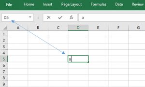
Opening an Excel spreadsheet. To open an Excel spreadsheet, find and press the Excel icon on your desktop. A blank worksheet should appear on your screen. Cells in Excel spreadsheets are identified with letter columns and row numbers. In Figure A.1, for example, the letter x appears in column D and row 5. When the cell with x is selected in the spreadsheet, the cell location is identified in the location tracker cell located in the top left of the spreadsheet as D5. (Try selecting different cells and observe the location tracker cell report the new location.)
Open Example in Microsoft Excel
Users can instruct Excel to perform operations on data in cells by entering a function or calling up an Excel supplied function. Users enter a function to be executed by first pressing the “=” sign. The “=” sign instructs Excel that what follows is a function to be executed.
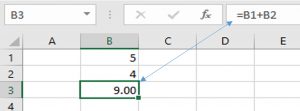
Entering user supplied functions in Excel. Excel has significant computing capacity that can execute user supplied functions. We illustrate a simple user supplied function in Figure A.2. We enter the numbers 5 and 4 into cells B1 and B2 respectively and in cell B3 instruct Excel to add the two numbers together. Note that the function appears to the right of the Excel function symbol fx on the blank space above the letters identifying the columns. After pressing enter, the function calculates the sum of 5 in cell B1 and 4 in cell B2 which is equal to the number 9 displayed in cell B3.
Open Example in Microsoft Excel
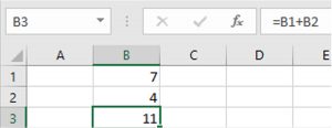
We can always recover the equation embedded in cell B3 by pointing the cursor to cell B3. One of significant advantage of Excel is that we can replace the numbers in cells B1 and B2 and the function will automatically recalculate their sum. To illustrate, in Figure A.3 we change the number 5 in cell B1 to 7. Excel uses the same function entered earlier to add cells B1 and B2 to return the sum of 11.
Open Example in Microsoft Excel
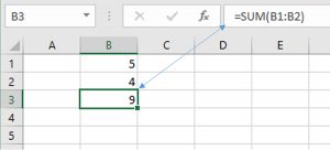
Excel’s library of functions. In addition to user supplied functions, Excel has a library of functions capable of operating on data identified in the spreadsheet. To illustrate, we employ Excel’s SUM function for adding numbers. The SUM function lists the location of the beginning and ending cell in the string of numbers to be added, separated by a colon. We use the SUM function to solve the example described in Figure A.2 by entering into cell B3 the function SUM(B1:B2).
Open Example in Microsoft Excel
Excel and handles. A “handle” is powerful Excel tool that enables Excel users to repeat operations or values in a cell by dragging the cell handle to a new location. In the new cell, the function in the handle cell is repeated and updated or the value in the handle cell is repeated. We describe handles next.
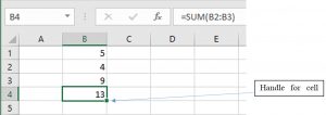
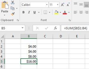
In Figure A.4, note the bold lines around cell B3 where the cursor is pointed. At the bottom right corner of the cell is a solid square called the handle. If we click on the handle and drag it to a new cell, B4, the function in cell B3 is repeated in cell B4, and the cell locations in the SUM function will be updated by one row value. In the other words, the function in the original cell SUM(B1:B2) is updated by one row in cell B4 to SUM(B2:B3). Just as the SUM function in cell B3 added the preceding two numbers, so does the SUM function in B4 add the preceding two numbers—4 and 9. We illustrate the use of handles in Figure A.5.
Open Example in Microsoft Excel
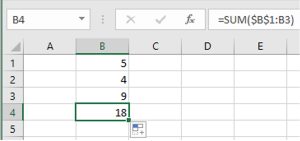
Fixed cells. The function in B3 was SUM(B1:B2), and the updated function in B4 was SUM(B2:B3). However, there may be occasions when we want to fix a cell’s location in a function rather than have it automatically updated when dragged. In our example, suppose that we wanted to add the string of numbers that began in cell B1 rather than having the addition begin with the number in cell B2 when dragged one cell. To do so, we merely fix cell B1’s location in our function by preceding the column letter and row number with a “$” sign as in $B$1. Other cells identified in the function that are not fixed are updated when the cell containing the function is dragged by its handle. In our example, the function in B4 updates the cell at the end of the string but keeps fixed the cell B1 at the beginning of the string. To illustrate, in Figure A.6 the SUM function contains a fixed cell B1 but updates the ending cell in the string when the function in B3 is dragged to location B4.
Open Example in Microsoft Excel
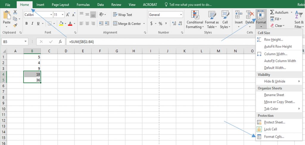
Formatting cells. Suppose we wanted to indicate that the numbers in the string and function reflect dollars (or percentages, etc.). For the cells to reflect dollar amounts, we must format the cells in the Excel. To format Excel spreadsheet cells, we click “Home” on the main ribbon and then click “Format” on the drop-down menu. Notice that the last entry in the drop down Format menu is labeled “Format Cells” (See Figure A.7.).
Open Example in Microsoft Excel
Lastly, we click on “format cells” and note the several format options. After we highlight the cells we wish to reformat, we click the currency line with two decimal places.
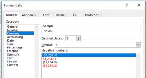
We display in Figure A.9 the numbers reformatted as currency.
Open Example in Microsoft Excel
Excel Financial Functions
Compound interest. We illustrate the important concepts of user supplied functions, handles, and fixed cell locations by calculating compound interest. Suppose we begin in the present, period zero, with an investment of $10,000 that earns 5% per period. Therefore, at the beginning of period 1, our original investment has grown to $10,000(1.05) = $10,500. If we allow the original investment plus interest to grow another period, we have at the beginning of period two an investment of $10,000(1.05)(1.05)=$11,025. It might be interesting, although tedious, to see how our investment would grow over 10 periods following the same procedure. Excel can easily solve this problem using cell handles.
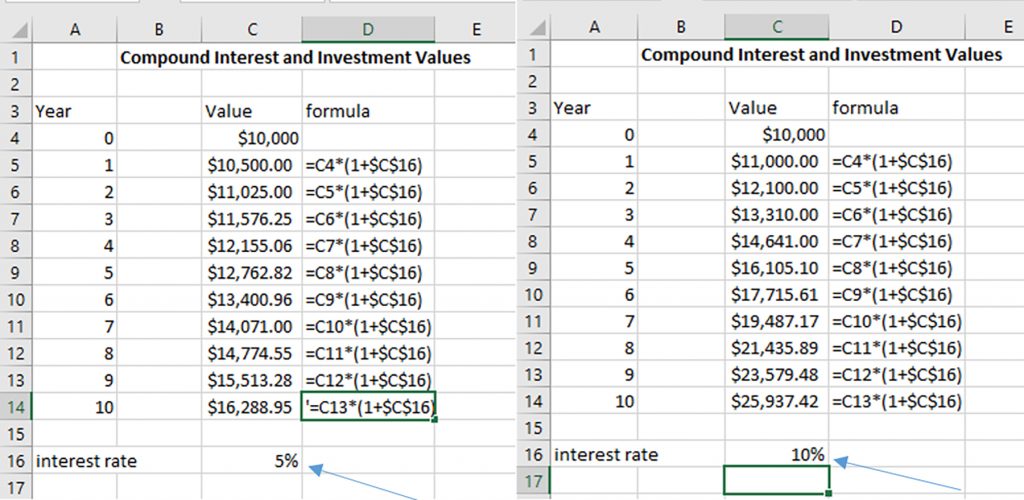
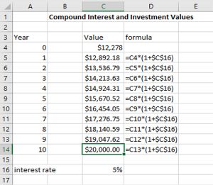
To begin, we label cell A3 “Years” and in cells A4 through A14, we list the number of years for which we want to compute the value of an investment that earns compound interest beginning in the present. We label cell B3, “Compound Values.” At the beginning of year 0 in cell B4, we list the original investment amount. At the beginning of year 1 in cell B5, we enter the function for compounding the value in the previous cell—multiplying the previous cell’s value by 1.05. Clicking on the handle in cell B5, and dragging it to year 10 in cell B14, we calculate the value of the investment in each of the 10 periods. To make clear this operation, we display the function in each cell to the right of the cell in which the function is embedded. If we wish to explore the effects of compounding with alternative interest rates, we change the interest rate listed in cell C16. For example, compare the investment’s value compounded at 5% percent rate compared to the investment’s value compounded at 10%. The comparison is reported in Figure A.10.
Open Example in Microsoft Excel
Goal Seek. In the previous example, we found that $10,000 compounded at 5% for 10 periods produced a value of $16,288.95 and $25,937.42 if $10,000 were compounded at 10%. Suppose our goal was to have $20,000 at the end of 10 years of compounding. We might ask: what initial investment, an exogenous variable, compounded for 10 years at 5% would produce a $20,000, an endogenous variable whose value is determined within the system? We could, of course, answer this question by experimenting with alternative investment values in cell C4 where the initial investment amount is stored. However, this would be tedious and may be difficult to find the exact amount.
Excel offers an alternative approach to finding the desired value of an endogenous variable by changing an exogenous variable using an algorithm called “Goal Seek.” Excel’s Goal Seek algorithm answers “what if” kinds of questions. Specifically, it answers the question “what if” the value of the endogenous variable located in a particular cell has some specified value, then what must be the value of the exogenous variable located in another designated cell? Excel records the new values for endogenous and exogenous variables in the Excel spreadsheet. We illustrate the process using the compounding investment example described in Figure A.10.
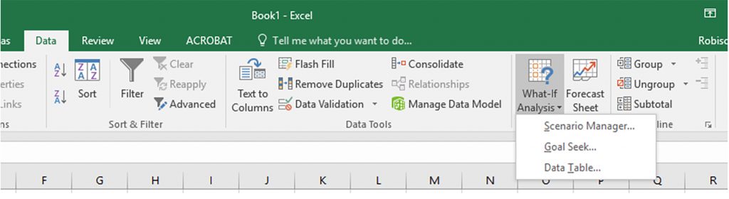
To access Goal Seek, press the [Data] tab and the [What If Analysis] button. Finally, press “Goal Seek…” in the drop-down menu. The Data tab, the What If Analysis button, and the drop-down menu displaying the Goal Seek option are displayed in Figure A.11.
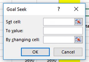
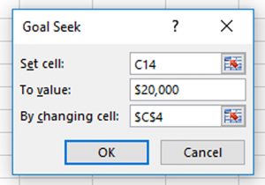
The Goal Seek dialogue box asks that the endogenous variable’s cell location be identified in the “Set cell” entry field. We enter the desired value of the endogenous variable in the “To value” field. Finally, we identify the cell location of the exogenous variable that is to be changed in the “By changing cell” entry field. After pressing “OK”, Goal Seek finds the value of the exogenous variable required to obtain the desired value of the endogenous variable.
To illustrate, suppose we wanted to have an investment value of $20,000 at the end of 10 years. Our “what if” question is: What if the value of our original investment compounded at 5% for 10 years were $20,000? Then what would be our required investment amount? To solve this problem, in the Goal Seek dialogue box we enter cell C14—the endogenous variable location—in the “Set cell” field; we enter $20,000 in the “To value” field; and we enter cell location A4—the exogenous variable—in the “By changing cell” field. The results are recorded in Figure A.13.
Pressing the “OK” button returns the Goal Seek solution reported in Figure A.14.
Open Example in Microsoft Excel
We have determined using Goal Seek that an investment value of $20,000 at the beginning of period 10 requires that we invest $12,278 in the present—an increase of $2,278 over the original investment.
An Application of Goal Seek to HQN’s Coordinated Financial Statements (CFS)
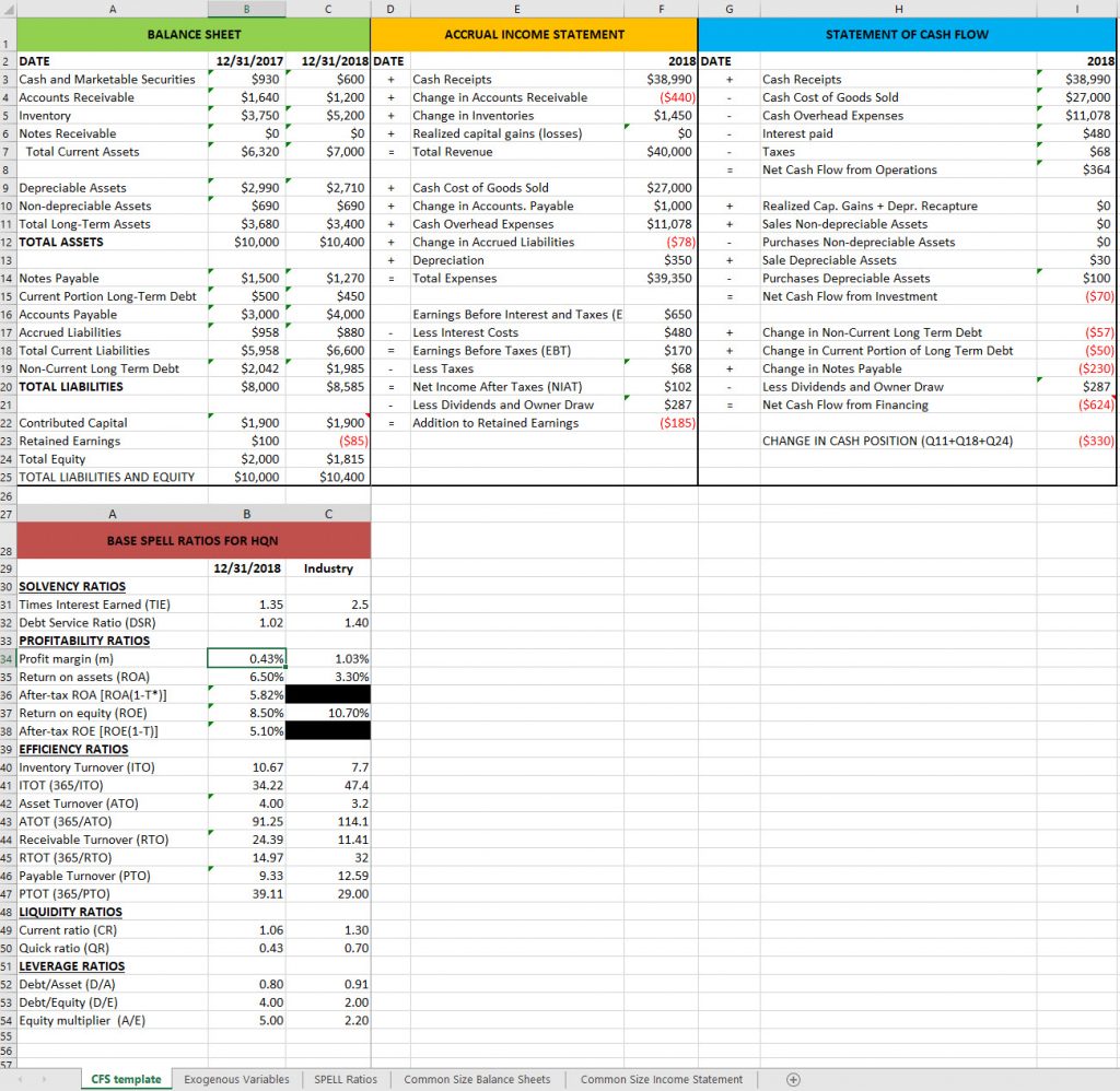
In the text, we explored HQN’s financial condition reflected by its CFS and associated ratios, DuPont equation, and common size balance sheet and income statements. We now use Goal Seek to find the value of an exogenous variable required to produce the desired value of an endogenous variable. To begin, we copy HQN’s original CFS in Figure A.15.
Open CFS Example in Microsoft Excel
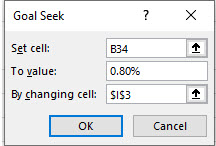
Now suppose we are concerned about the low cash receipts efficiency ratio m and ask: what must our cash receipts equal to produce an m efficiency ratio of .8% or 8/10th of a penny on each dollar of sale? To answer this question, we enter the following into our Goal Seek dialogue box.
After pressing OK, we return the answer to our “What if” question in figure A.17.

Open “What if” CFS Example in Microsoft Excel
The Goal Seek answer to the “what if” question described earlier is that cash sales must increase to $39,142 in order for HQN to produce an m ratio equal to .8%. We may also observe that the new level of cash receipts would also increase both ROA and ROE values to well above industry standards. The ROE ratio increases from 8.5% to 16.11%. The ROA increases from 6.50% to 8.02%. Furthermore, increased cash receipts would improve the debt-to-service ratio from 1.02 to 1.18.
An overview of financial functions.
This section discusses how to use Excel financial functions, some of which were discussed in earlier book chapters—particularly Chapter 17 on loan analysis. Obviously, the financial functions discussed in this section are only a sampling of the many financial and other functions available to Excel users. We begin by writing the general present value (NPV) function in equation A.1. The various financial functions we will discuss in what follows are only special cases of equation A.1.
(A.1) 
We begin by noting a fundamental algebraic reality. A single equation can solve for at most one unknown variable—although the unknown variable may have more than one solution. Therefore, equation A.1 can produce a solution(s) for at most one unknown. As a result, all of the financial models described in this appendix assume that one of the variables in equation A.1 is unknown. Consider the following financial models that result by assuming one of the variables in A.1 is unknown.
The net present value (NPV) model. The NPV model solves for the net present value of an investment, the present value difference between the cost of the investment V0 and future cash flows discounted by rate r/m plus the investment’s liquidation value Vn.
The internal rate of return (IRR) model. The IRR model finds the value of the discount rate r that makes NPV equal to zero. The variable r is unknown, and because it enters the equation with an exponent, r may have more than one solution.
The maximum bid (minimum sell) price model. The maximum bid price model finds the value of V0 such that NPV is zero. It represents the most an investor could pay for a future cash flow stream and still break-even. The value of V0 that makes NPV zero may also represent the least-price an investor could receive in exchange for the investment’s future cash flow stream and still break-even.
The annuity equivalent (AE) model. There are two versions of the annuity equivalent model. The first one finds the value of a constant cash flow R received for mn periods whose NPV equals the present value sum of cash flows Ri(i = 1, …, mn) plus Smn, the equation’s NPV.
(A.2) 
In the second version of the annuity equivalent model, we set NPV equal to zero and find the annuity equivalent whose discounted value is equal to V0. Cash flows associated with a constant loan payment fit this model where V0 is the loan amount, R is the constant loan payment, r/m is the interest rate, and mn is the term of the loan.
(A.3) 
Break-even models. In some cases, we might be interested in a particular value of Ri or the liquidation value Smn that reduces NPV to zero. In these cases, we often employ Goal Seek to find that particular Ri or Smn value.
The term model. There are two term models considered in this book. In the first, the unknown variable is the term, mn, and its solution depends on the other known variables in the equation. In the second term model, called the optimal term model, the solution for mn depends on a calculus-defined condition requiring that we solve the model for various values of mn until the optimal conditions are satisfied. This is a difficult model to solve because it requires that we know additional future values of variables. Forecasting the future values of variables is discussed in Chapter 11.
The future value model. The future value model solves for Smn, the liquidation value of the investment, assuming NPV is equal to zero. The uniqueness of this model is that instead of discounting future cash flows to their present value, we compound cash flows to their future value in the mnth period
Excel functions.
Corresponding to the general NPV equation variables described in A.1 are several Excel functions. Excel’s PV function finds NPV and V0. Its PMT function finds R, an AE. Its NPER function finds mn. Its RATE function finds r/m, and its FV function finds the value of Smn after setting NPV equal to zero.
Corresponding to the Excel functions PV, RATE, NPER, PMT, and FV are the arguments pv, rate, nper, pmt, and fv. Functions are capitalized. Arguments corresponding to functions are lowercased. When we solve for a particular function, the corresponding argument is eliminated from the function’s list of arguments. We list the following Excel functions, their arguments, and the order in which the arguments appear. In addition to the list of arguments, functions call for “type” variables which tells the function whether cash flows occur at the beginning of the period in which case type=1 or at the end of the period in which case type=0. If values are not entered for “type” and “fv”, Excel assumes they are both equal to zero. Excel financial functions and their arguments are listed next.
- The PV function is =PV(rate, nper, pmt, fv, type).
- The FV function is= FV(rate, nper, pmt, pv, type).
- The RATE function is =RATE(nper, pmt, pv, fv, type).
- The NPER function is =NPER(rate, pmt, pv, fv, type).
- The PMT function is =PMT(rate, nper, pv, fv, type).
To solve the functions listed above, we enter the cell locations of the argument values and enter them into the Excel function. For example, if the value for rate were listed in cell C4, nper were listed in cell C5, pmt were listed in cell C6, and fv and type were both zero, we would write the PV function as =PV(C4, C5, C6, 0, 0).
Calling up Excel Functions.
There are two ways to call up Excel functions. The first way is to write the function with its argument values in a designated location. For example, assume the value for rate were listed in cell C4, nper were listed in cell C5, pmt were listed in cell C6, and fv and type were both zero and listed in cells C8 and C9. Then, we would write the PV function in cell C7 as =PV(C4, C5, C6, C8, C9).
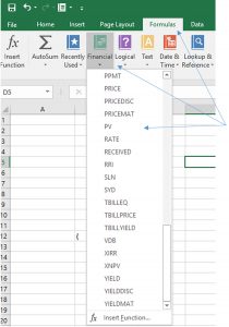
A second way to call up an Excel function, particularly if the name of the function or its arguments are not known, is to click on the Formulas tab on the main ribbon and the Financial button that produces a drop-down menu with a list of financial functions. The financial functions NPER, RATE, PV, FV, and PMT are included in the list. To illustrate, we find and click the PV function in Figure A.18 below.
After clicking on PV in the drop-down menu, the PV function dialogue box with its list of arguments is displayed in Figure A.19.
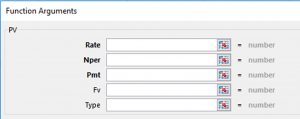
To review, the PV function arguments correspond to variables in equation A.1. Rate corresponds to “r/m”, the discount rate in an NPV model or the interest rate in a constant loan model. Nper corresponds to the product of mn, the number of periods we compound interest in equation A.1. Pmt corresponds to the annuity equivalent R. FV corresponds to future value. One other argument not explicitly described in equation A.1, type, identifies if cash flows occur at the beginning of the period, in which case we enter the number 1, or if calculated at the end of the period, in which case we enter the number 0.
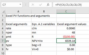
To illustrate, we solve for pv using the PV function. We begin by listing value for all of the PV arguments and in the cell that calls for a pv value, we enter the PV function. Our example in Figure A.21 corresponds to the example in Chapter 17. The annual percentage rate r equals 5%. The number of compound periods per year m is 12. The number of years n is 4. And the annuity equivalent R entered with a negative sign is –R = –150. We now transform the numbers corresponding to equation A.1 into PV function arguments. Rate equals r/m = .05/12=.004; Nper equals mn = 12 x 4 = 48. In cell C7 we enter the function PV with its arguments. For the first argument of the PV function we list the location of rate in cell C4. The second argument of the PV function is nper located in cell C5. The third argument is pmt located in cell C6. The fourth argument is pv in cell C7. Since pv is an endogenous variable in the PV function, we enter the PV function is cell C7. Finally, type is equals to zero in cell C8 and fv is also zero located in cell C9. The PV formula in cell C7 is expressed as =PV(C4, C5, C6, C8, C9). The solution to the PV equation with argument values described in Chapter 17 and repeated above are illustrated in Figure A.20.
Open Example in Microsoft Excel
Notice that the argument values for the PV function are listed in cells C4, C5, C6, C8, and C9. The unknown (endogenous variable) pv is located in cell C7. So in cell C7 we list the PV function and its arguments described in the function box located at the top of the figure.
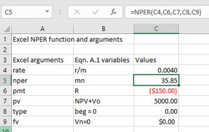
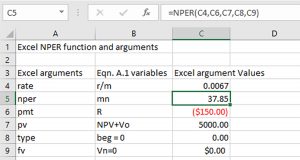
To illustrate another function, suppose that we knew that pv=$5,000 but that nper was unknown. In which case we would enter $5000 in cell C7 and enter the NPER function in cell C5: =NPER(C4, C6, C7, C8, C9). The solution is described in cell C5, and the NPER function is entered in the function box. These results are described in Figure A.21.
Open Example in Microsoft Excel
Of course, we can explore “what if” questions by changing arguments values of the function NPER and noting the consequences on nper. For example, what if we change the variable r in cell B4 to 8% so that r/m = 8% / 12 = .0067. Then we ask, what is the new value of nper? The worksheet with the revised value for rate is described in Figure A.22.
Open Example in Microsoft Excel
To this point, we have assumed time varying cash flows in equation A.1 have been replaced by their AE equal to R. But in some cases, it is important to consider the time varying cash flow rather than the AE cash flow. Excel’s NPV function allows us to do just that—consider time varying cash flows. Excel’s NPV and IRR function considers the complete A.1 equation including its time varying cash flow.
The NPV function. The NPV function has only two arguments: the rate argument and the stream of periodic cash flows that can be entered individually separated by commas or entered as the first and last value in the cash flow stream beginning in period 1 and ending in period mn separated by a constant. The original investment value is not included in the function but added separately to the function value. We illustrate the NPV function using data from the Green and White Services investment problem.
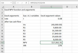
Green and White Services wants to know the NPV of an investment of $40,000 in lawn care equipment with expected cash flow during its four years of operation equal to: $9,800, $16,200, $17,840, and $19,600. In period five, Green and White intend to liquidate their investment and receive an after-tax cash flow liquidation value of $8,000. We enter these values in Figure A.23 and point the cursor at cell C12 where the NPV function is inserted. The first argument of the function is the discount rate of 8% recorded in cell C4. The second argument is the periodic cash flow in cells C7 through C11 separated by a colon. To the NPV function value we add the investment amount of ($40,000) located in cell C6. After pressing enter, the NPV function returns an NPV value of $17,061.91.
Open Example in Microsoft Excel
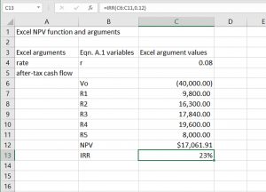
The IRR function with time varying cash flows. The IRR function finds the discount rate such that NPV is zero. The IRR function has only two arguments. The first argument is investment value. The second argument is the stream of periodic cash flows that can be entered individually separated by commas or entered as the first and last value in the cash flow stream beginning in period 1 and ending in period mn separated by a constant. We illustrate the IRR function using data from the Green and White investment problem. We enter the investment value in cell C6 and periodic cash flows in cells C7 through C11. We enter the IRR function is cell C13. Its first argument is the initial investment of ($40,000). The second argument is the periodic cash flow in cells C7 through C11 separated by a colon. After pressing enter, the IRR function returns an IRR value of 23%. We summarize this IRR example in Figure A.24.
Open Example in Microsoft Excel
Excel spreadsheets provide a powerful means for computing what otherwise would be tedious calculations. However, their ability to provide solutions to complex equations rapidly and repeatedly allows for a potential problem. The problem is that we may not spend sufficient time and effort to carefully specify the calculations we need Excel to perform. Cars are valuable means of getting us from point A to point B, but we still need to know the location of point A and point B. Excel spreadsheets provide valuable solutions to complex equations, but we still need to carefully define the problem to be solved and carefully derive the appropriate equation that solves the problem. Then, we are ready to enjoy the benefits of powerful Excel spreadsheets and formulas.
- The figures in the Appendix are screenshots of Microsoft Excel worksheets. The links to open Figures A.1, A.2, A.3, A.4, A.5, A.6, A.7, A.9, A.10, A.14, A.20, A.21, A.22, A.23, and A.24 all open the same Excel file. The worksheet tabs at the bottom of the Excel window can be selected for each figure. ↵
