List of Figures

Financial Management and the Firm

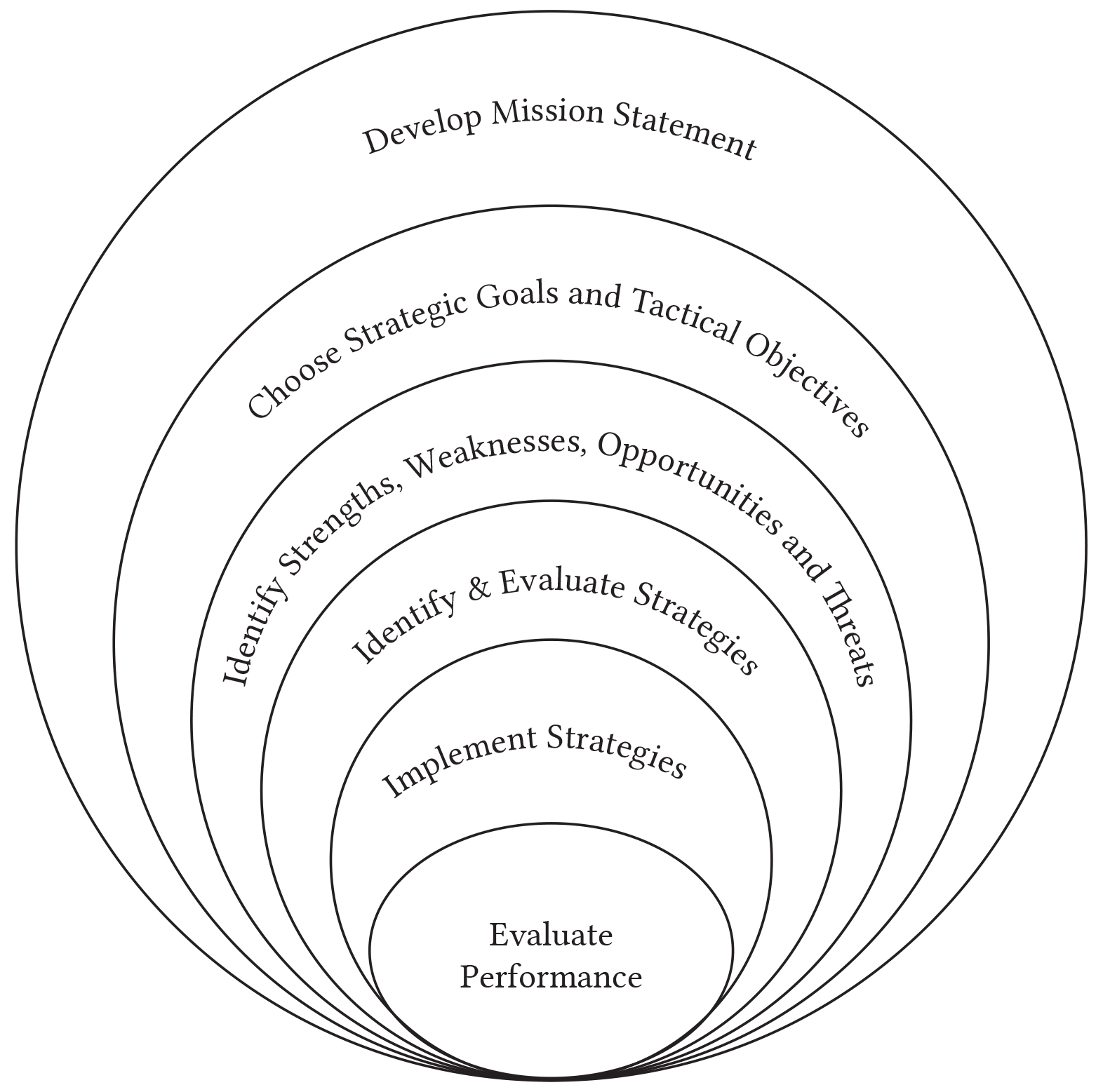
• Figure 1.1. The Managerial Process in Six Steps

Managing Risk

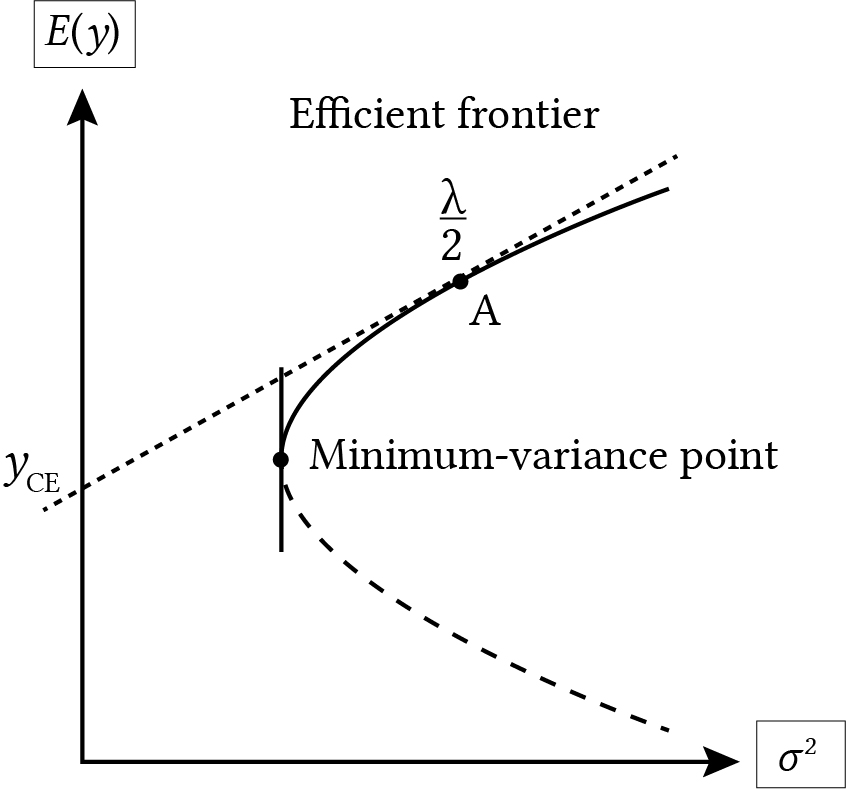
• Figure 4.1. An Efficient Expected Value-Variance Frontier of Investments Represented by their Expected Values E(y) and Variances σ².
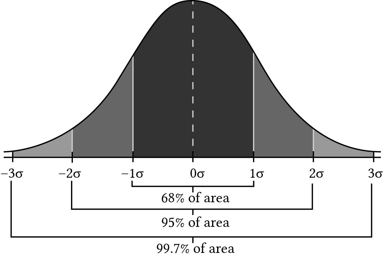
• Figure 4.2. A normal probability distribution that describes probability in areas divided to standard deviations from the mean.
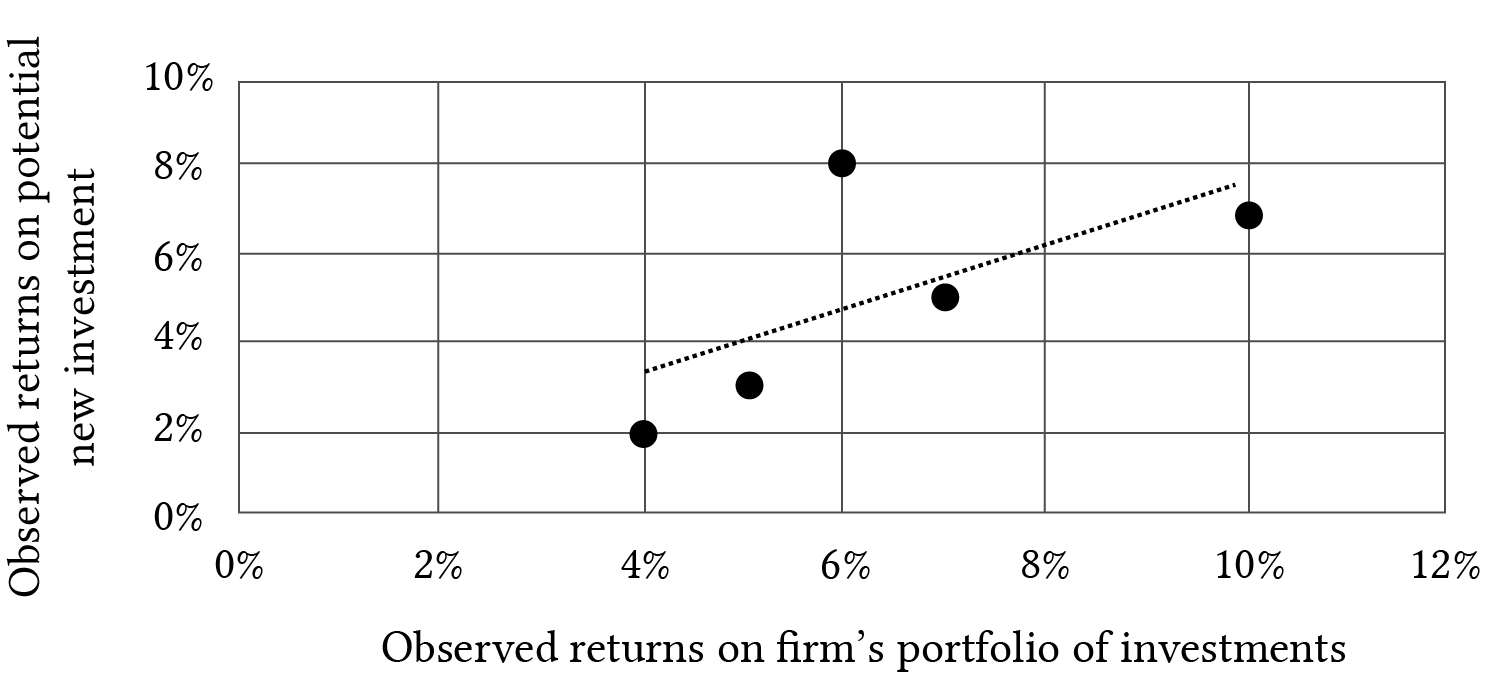
• Figure 4.3. Scatter Graph of Returns on the Firm’s Portfolio of Investments and Returns on the Potential New Investment

System Analysis

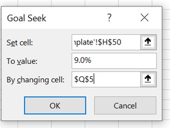
• Figure 7.1. Goal Seek Pop-up Menu

Incremental Investments

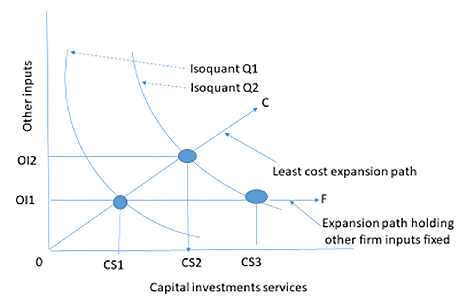
• Figure 10.1. Isoquants

Forecasting and Present Value Models

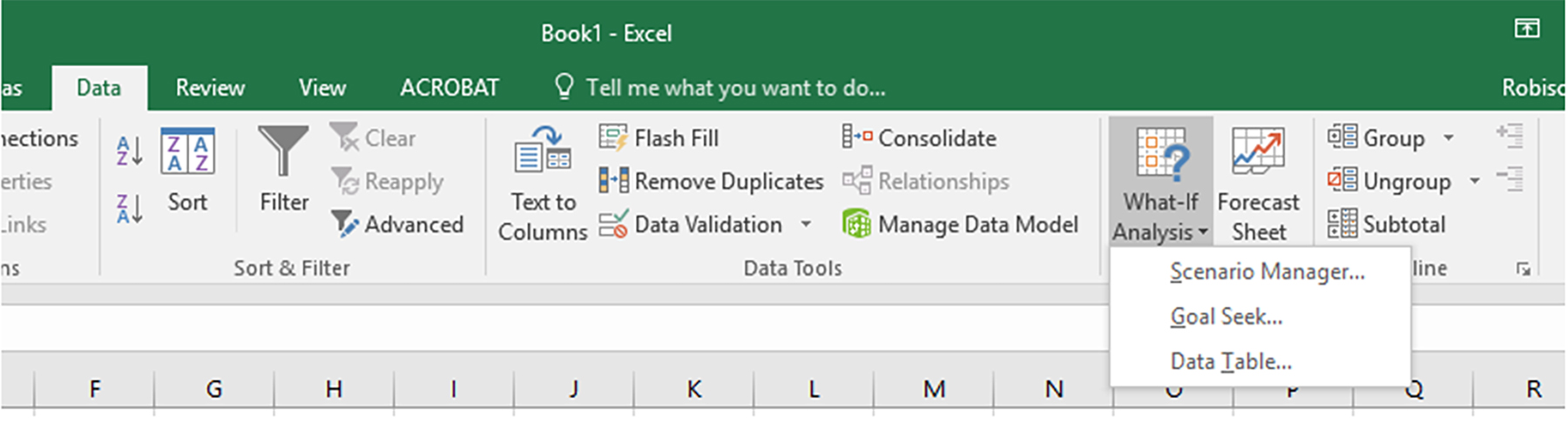
• Figure 11.1. Ribbon for Excel Spreadsheet
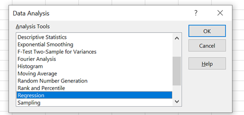
• Figure 11.2. Drop-down menu from the data tab.
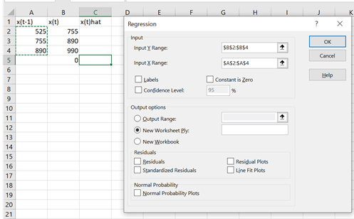
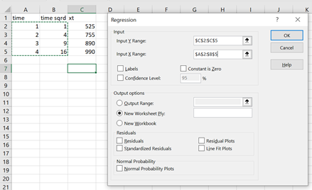
• Figure 11.3. Data input page for the regression analysis.
• Figure 11.4. Quadratic trend line.
• Figure 11.5. Data input page for a quadratic trend line.
• Figure 11.A1. Excel Data Menu Ribbon without the Data Analysis option.
• Figure 11.A2. Excel File Menu Options Selection
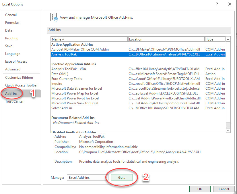
• Figure 11.A3. Excel Options to Manage Add-ins.
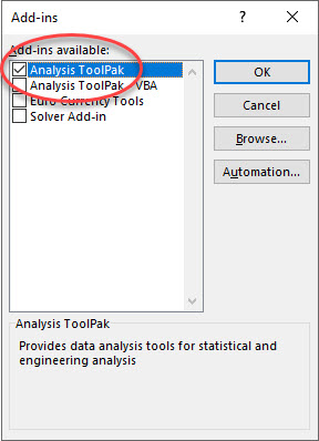
• Figure 11.A4. Enable Analysis Toolpak.
• Figure 11.A5. Data Ribbon with Data Analysis option enabled.

Homogeneous Liquidity and Currency

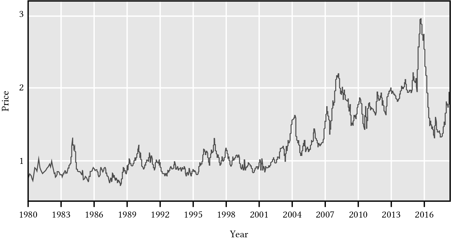
• Figure 16.1. The price of a dozen large eggs over the period 1980 to 2016. (Bureau of Labor Statistics, 2016)
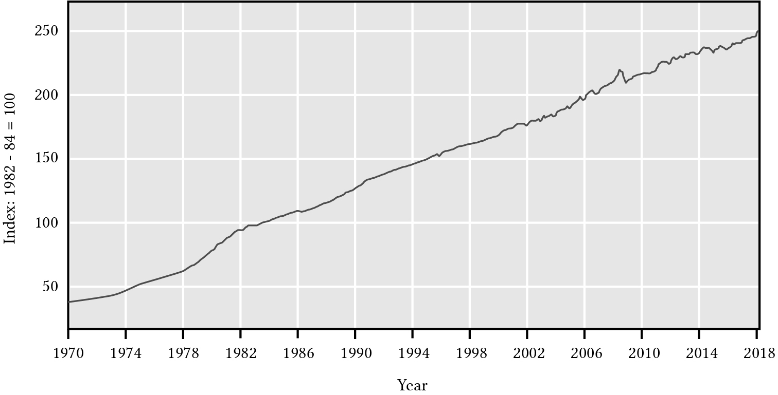
• Figure 16.2. The consumer price index for all the U.S. letting average prices between 1982-84 equal 100.
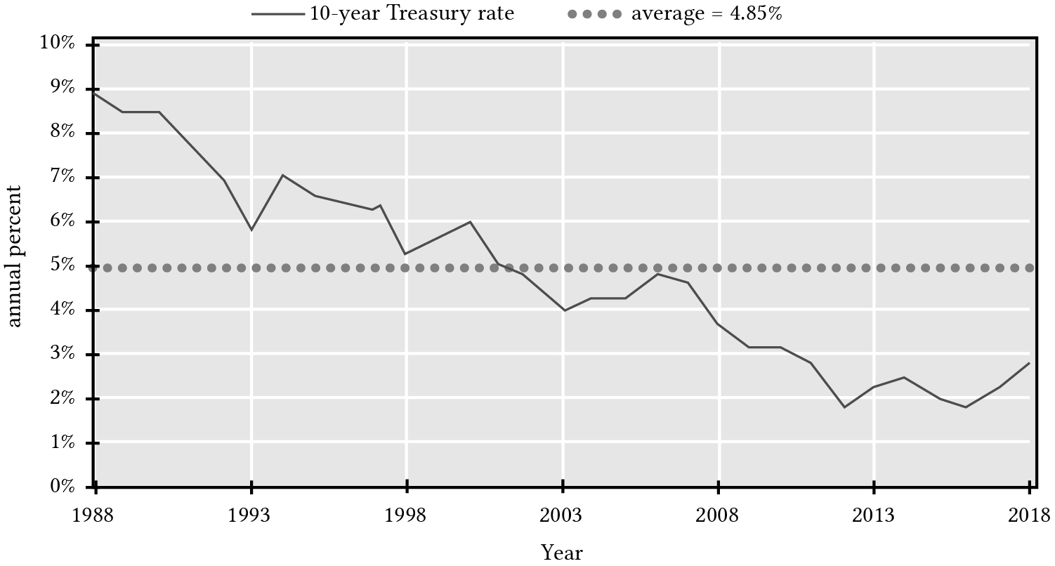
• Figure 16.3. 10-year Treasury constant maturity interest rate, U.S., 1988 – 2018
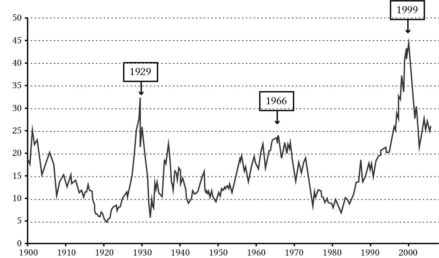
• Figure 16.4. Historic PE ratios for stocks described on the Standard and Poor’s Stock Exchange. (Earnings are estimated based on a lagged 10-year average.)
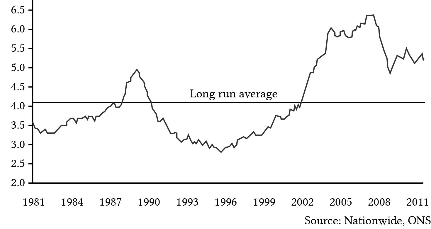
• Figure 16.5. Historic PE ratios for UK housing stock.
• Figure 16.6. Exchange Rate: Pound Sterling to US Dollar

Loan Analysis

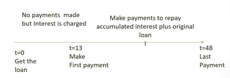
• Figure 17.1. The payment timeline for a 12-month skip payment loan with three years of payments.

Land Investments

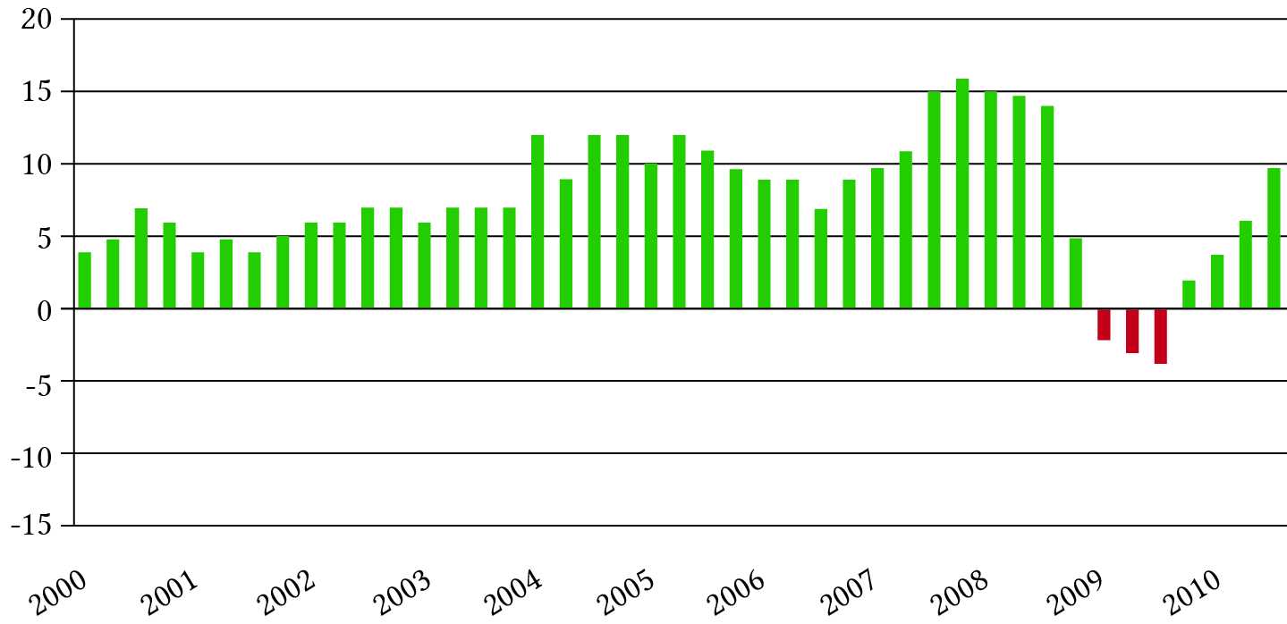
• Figure 18.1. Year-to-year changes in farmland values.
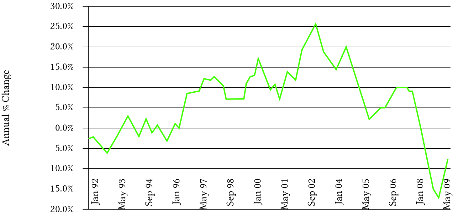
• Figure 18.2. Year-to-year changes in housing prices.
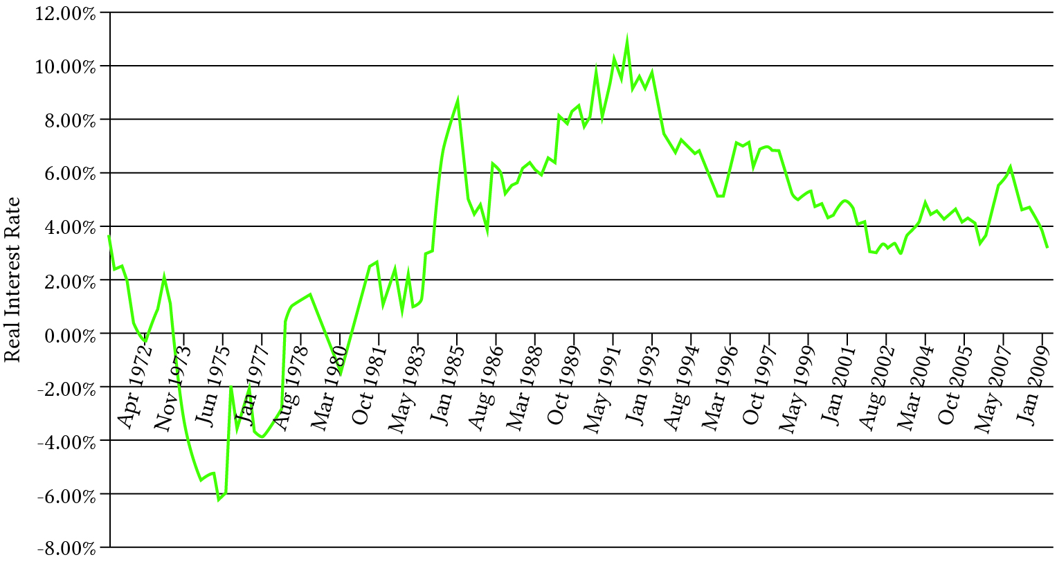
• Figure 18.3. Real home loan interest rates.
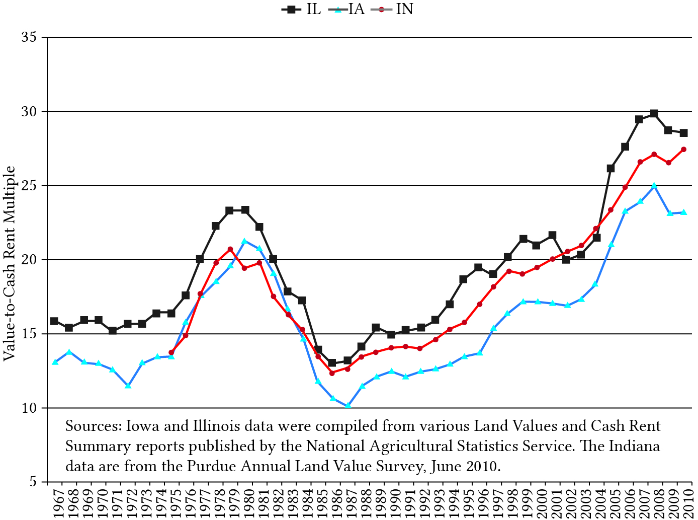
• Figure 18.4. Land values to rent ratios for land in Iowa, Illinois, and Indiana since 1967

Financial Investments

• Figure 20.1. Dow Jones crash in 2008.

Yield Curves

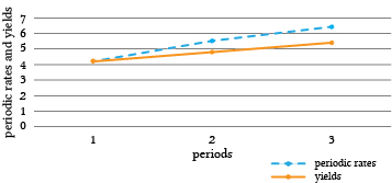
• Figure 21.1. A comparison of periodic interest rates and the corresponding yield curves of bonds of varying maturities
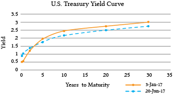
• Figure 21.2. Yield curves using U.S. Treasury debt calculated on January 3, 2017 and June 20, 2017

Econs and Humans

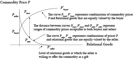
• Figure 22.1. Combinations of Commodity Prices and Relational Goods that Leave Buyers’ and Sellers’ Well-Being Unchanged.

Appendix

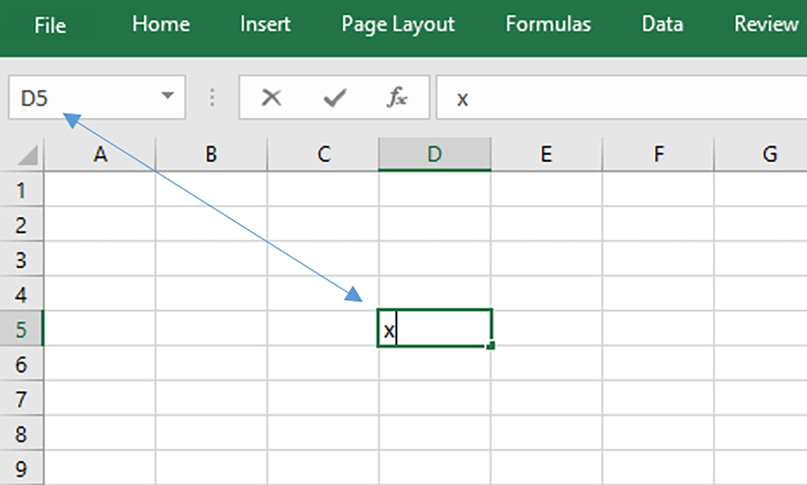
• Figure A.1. Identifying cell locations in Excel
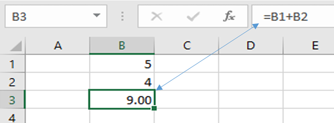
• Figure A.2. A user supplied addition function.
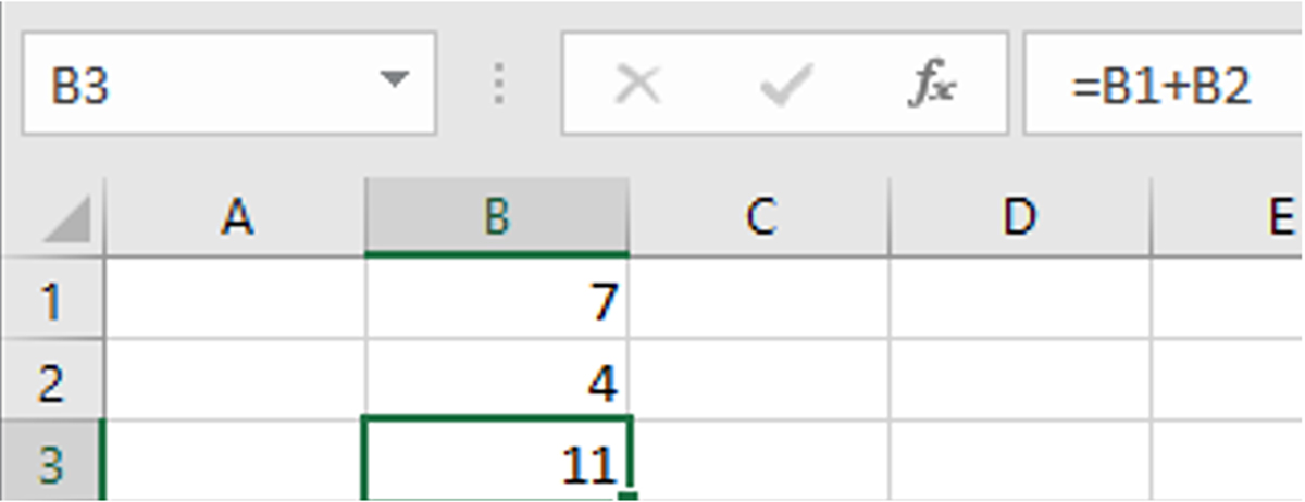
• Figure A.3. An Externally supplied addition function with a changed entry.
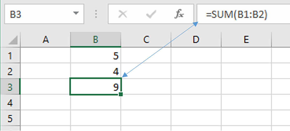
• Figure A.4. Adding numbers using Excel SUM function.
• Figure A.5. Dragging the handle in cell B3 to enter the same updated function in cell B4.
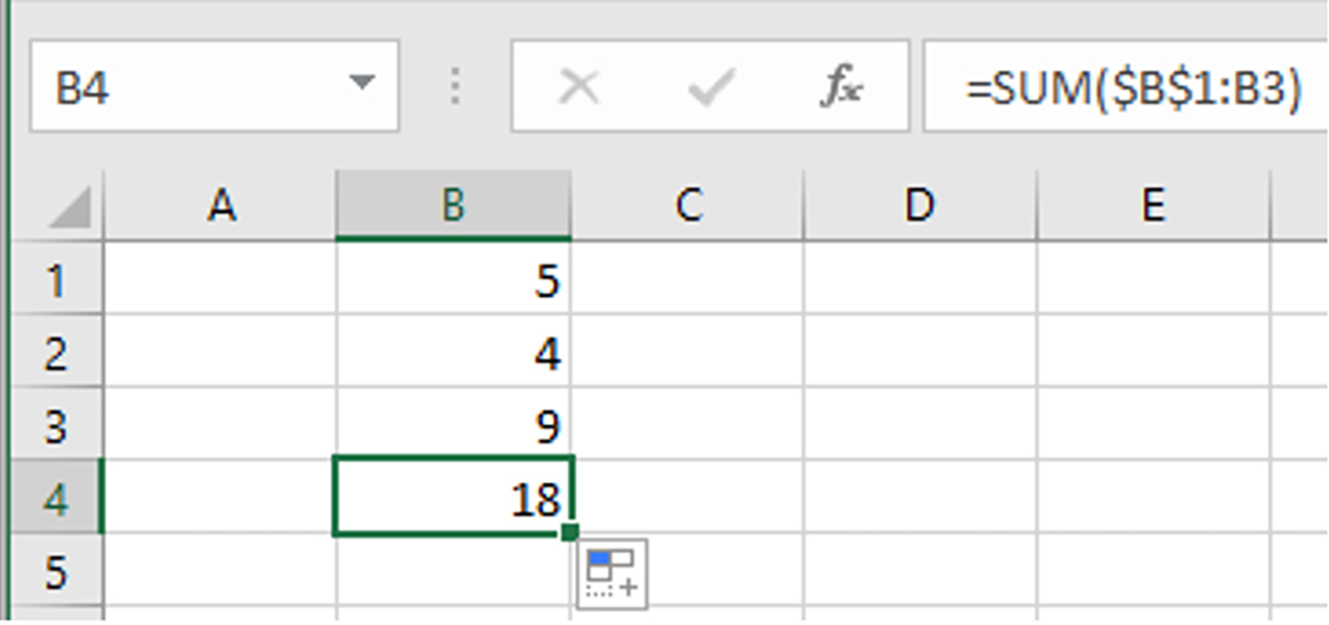
• Figure A.6. Using Excel’s SUM function to add a string of numbers with the number in the first cell fixed.
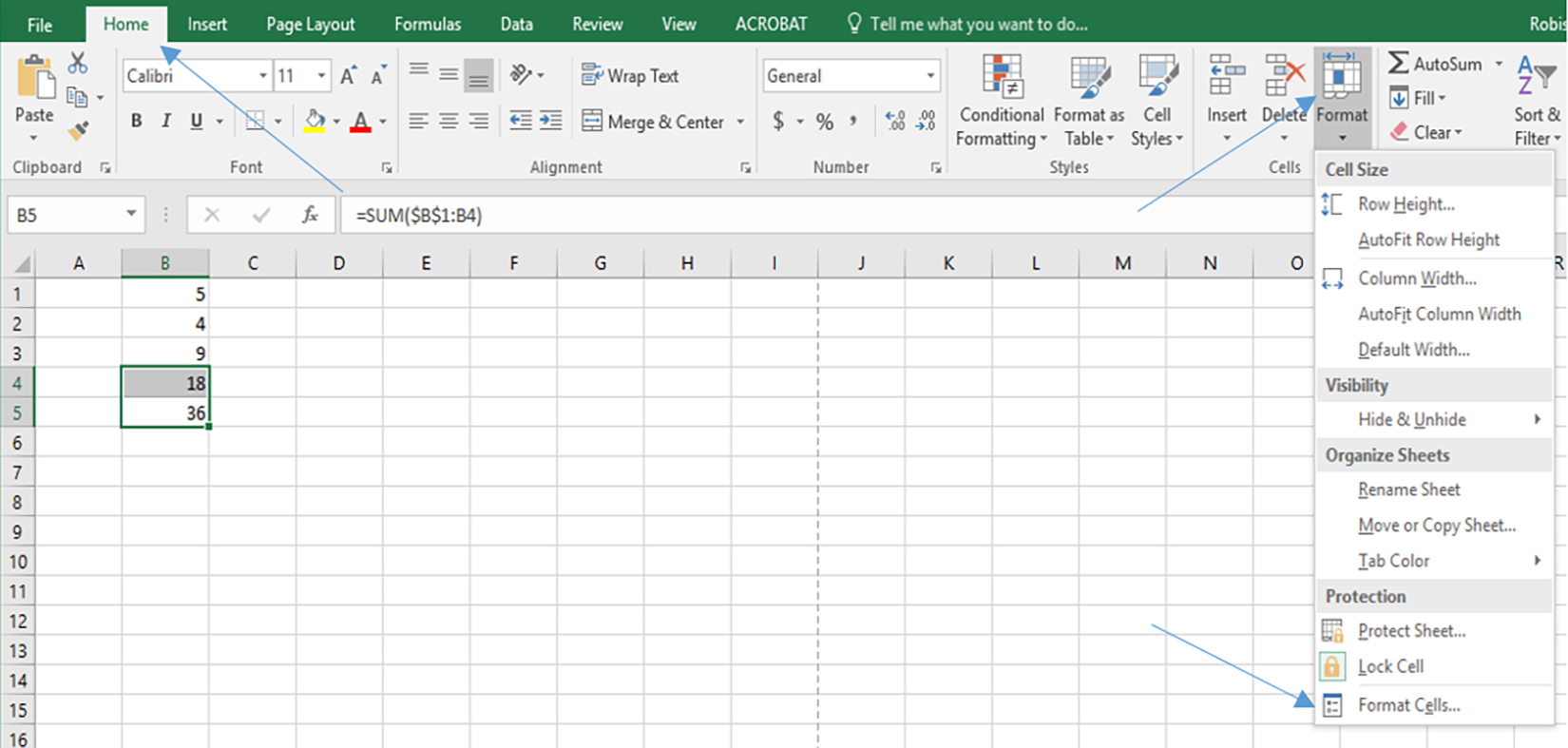
• Figure A.7. Formatting cells in Excel by accessing the Format cell options.
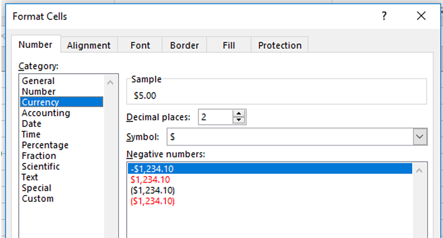
• Figure A.8. Cell formatting options.
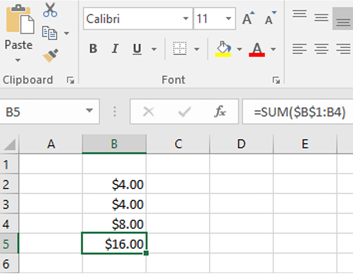
• Figure A.9. Currency Formatted cells
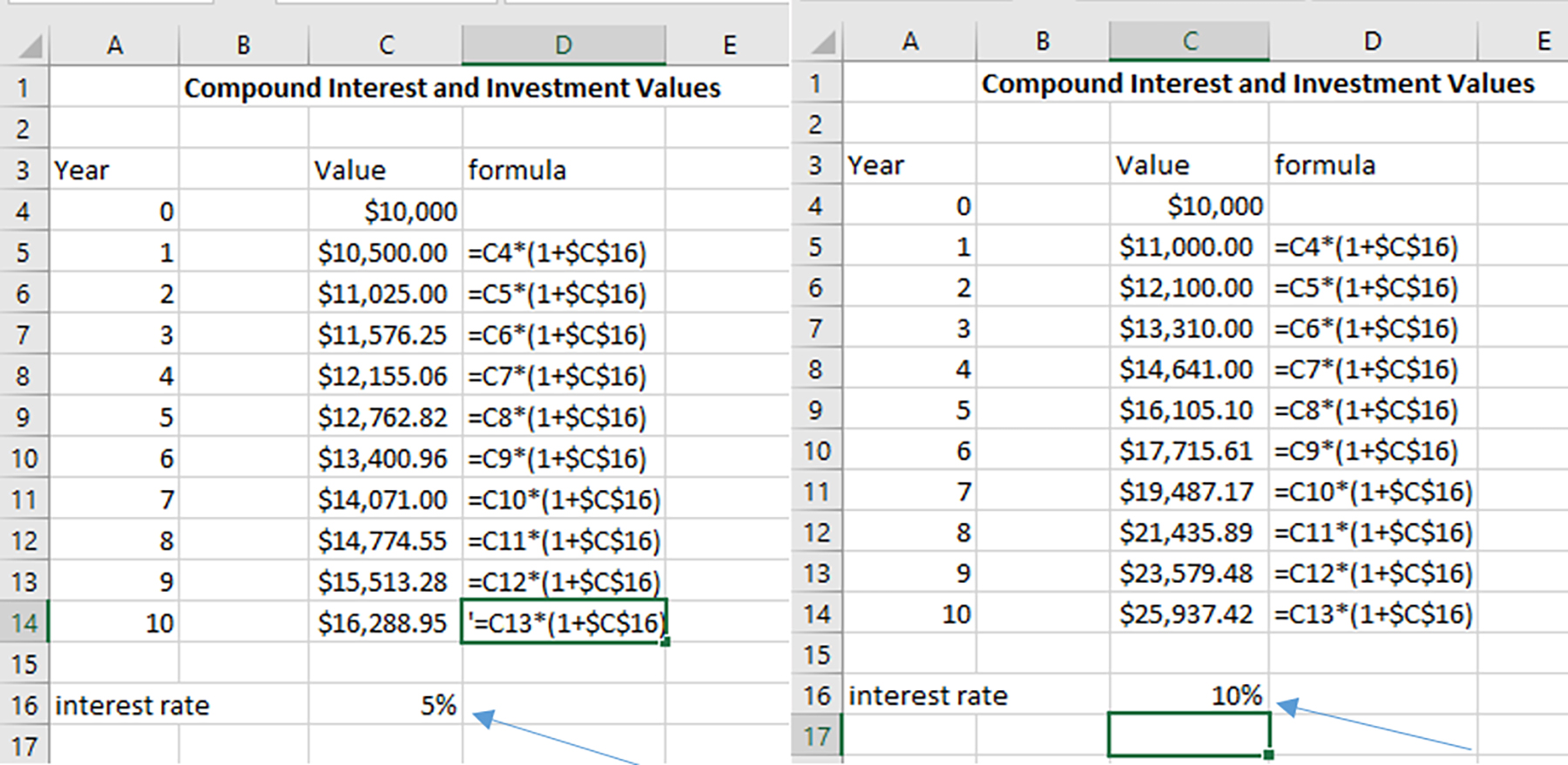
• Figure A.10. Analyzing the Effect of a 5% and a 10% Compound Interest Rate on Investment Values
• Figure A.11. Accessing Goal Seek in an Excel spreadsheet
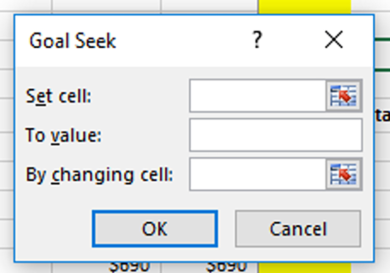
• Figure A.12. The Goal Seek dialogue box asking for the endogenous variable location to be recorded in the “Set” field, the desired value of the endogenous variable to be recorded in the “To value” field, and the location of the exogenous variable to be recorded in the “By changing” field.
• Figure A.13. A Completed Goal Seek dialogue box that instructs Excel to find the original investment compounded at 5% required to produce a $20,000 investment value at the beginning of period 10.
• Figure A.14. The Goal Seek solution, $12,278, equals the initial Investment compounded at 5% required to produce a $20,000 value at the beginning of period 10.
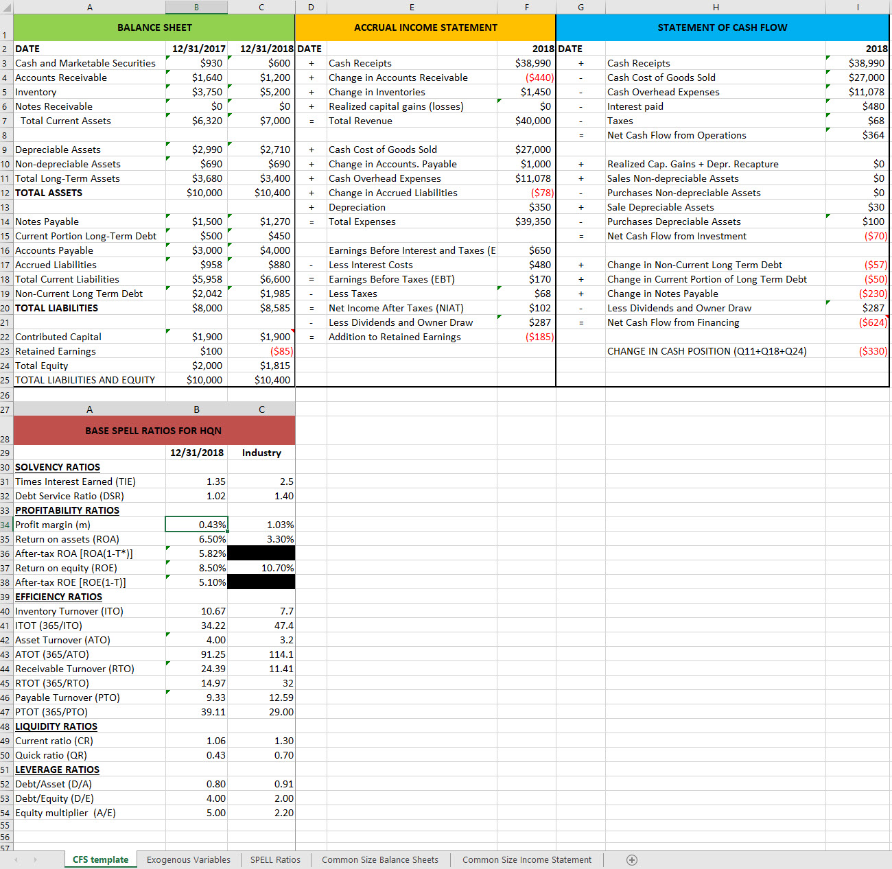
• Figure A.15. HQN’s Coordinated Financial Statements and Embedded Functions and Associated Ratios
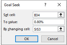
• Figure A.16. Solving the “What if” question, how much does cash receipts need to increase to obtain an m ratio of .8% using Goal Seek
• Figure A.17. The Goal Seek solution to the “What if” question, how much will cash receipts need to increase to produce an m value of .8%?
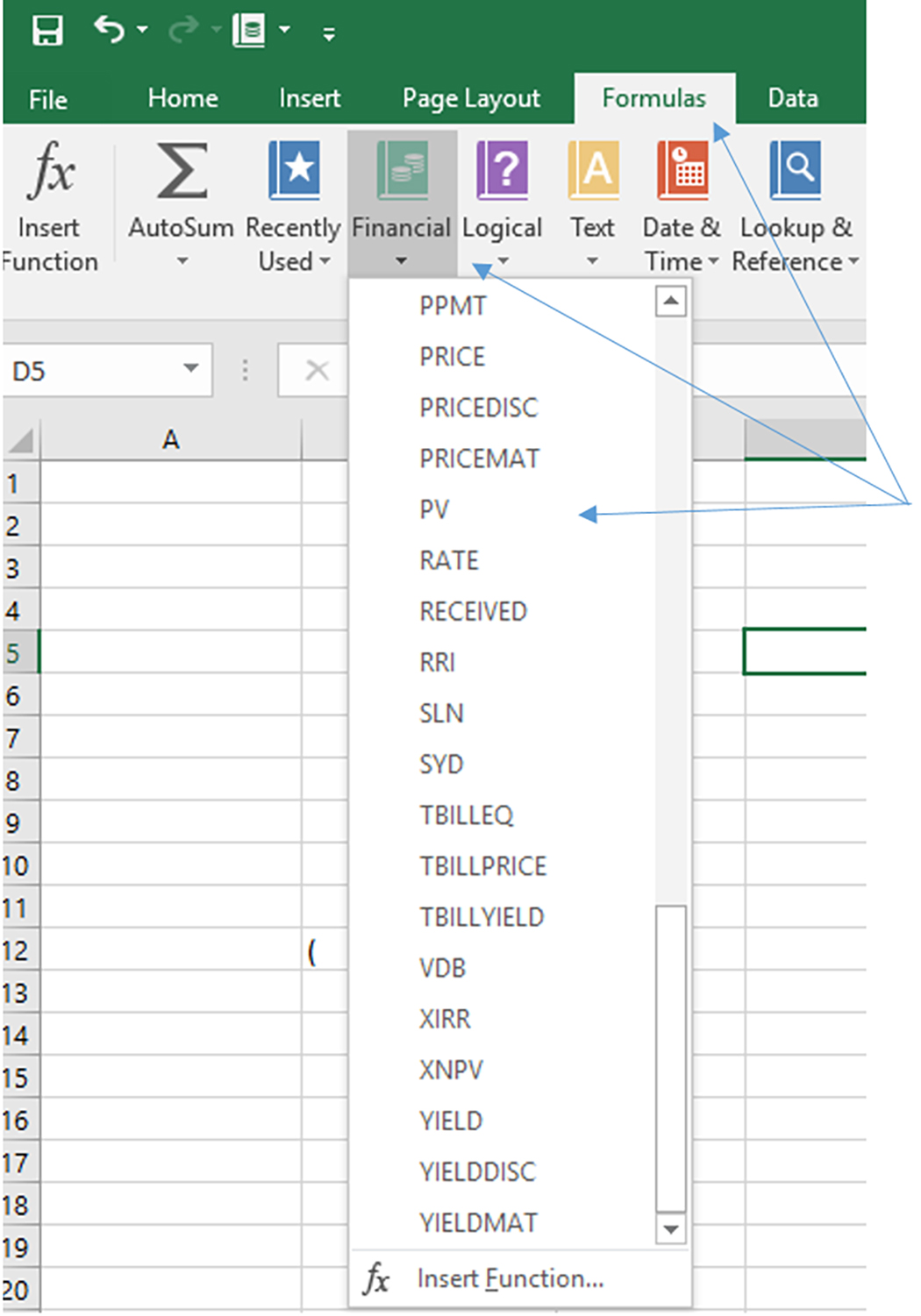
• Figure A.18. Opening the Excel PV function.
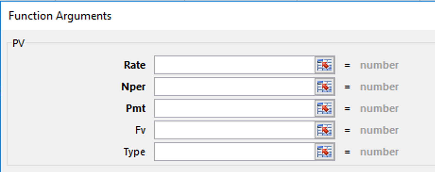
• Figure A.19. The PV functions and its arguments.
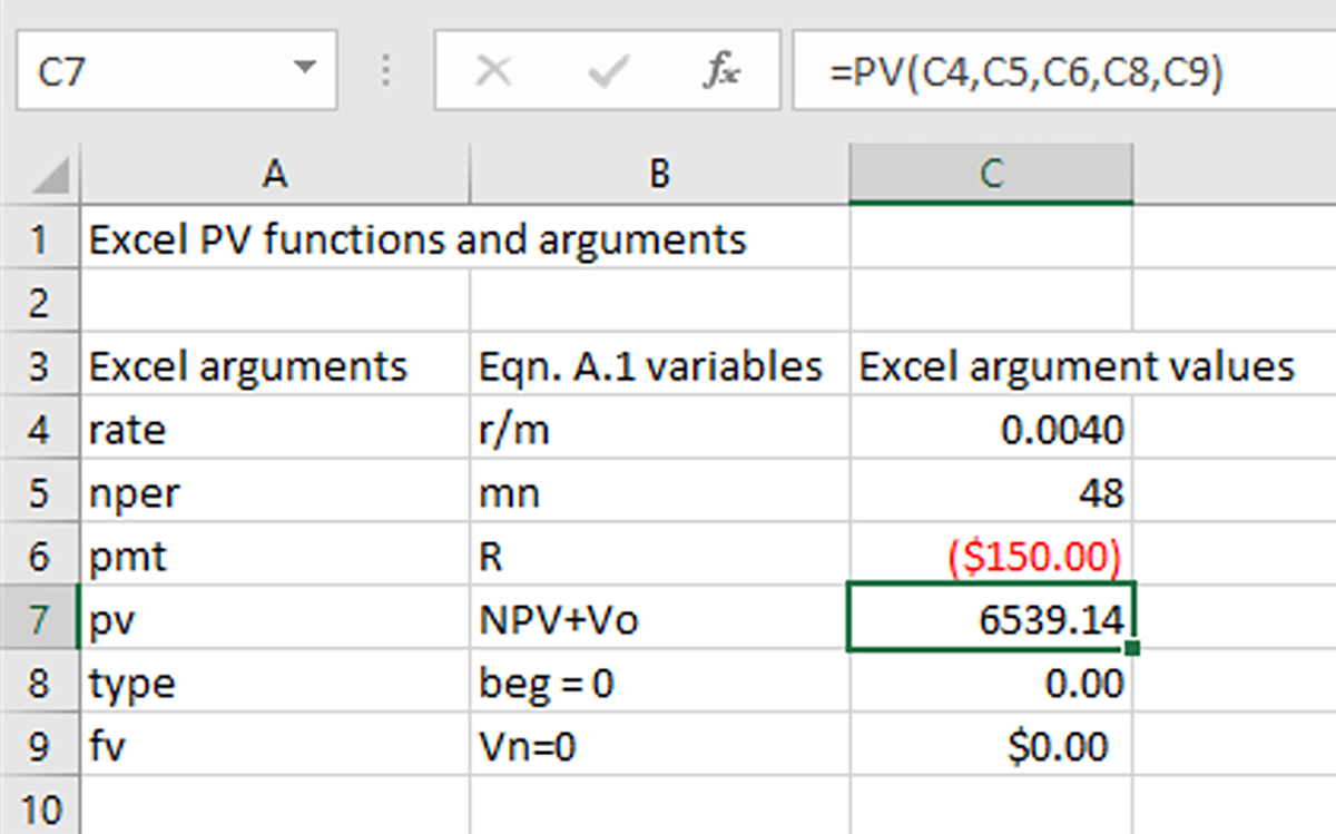
• Figure A.20. An Excel PV function solution for equation A.1 where A.1 variables are described in cells C2 through C7.
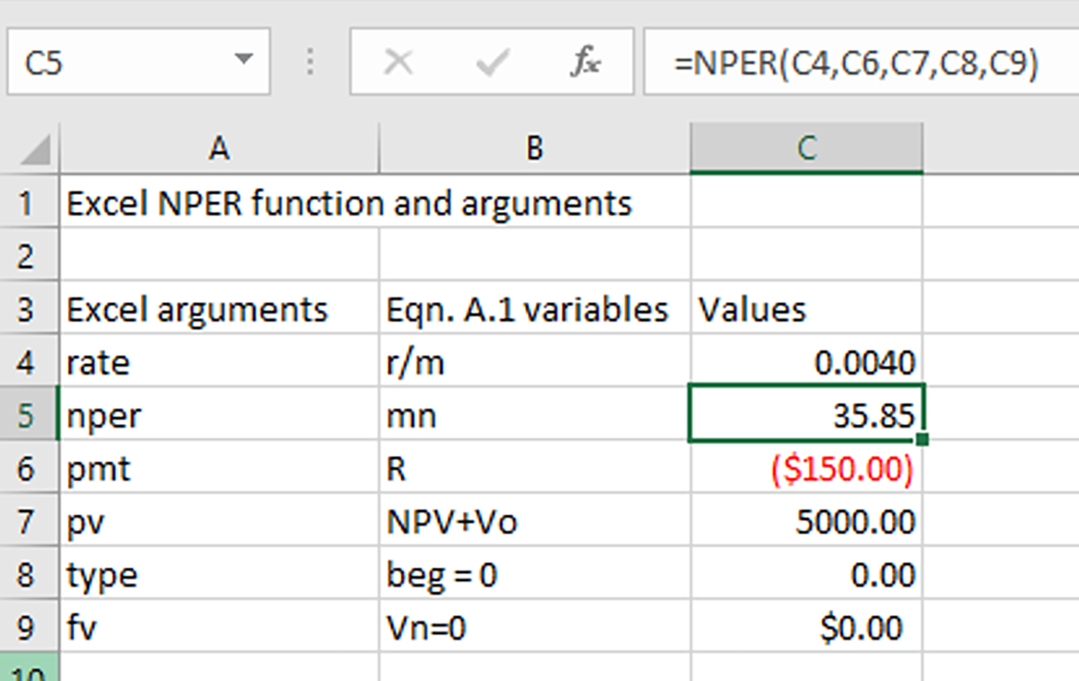
• Figure A.21. Answering the “what if” the nper was unknown.
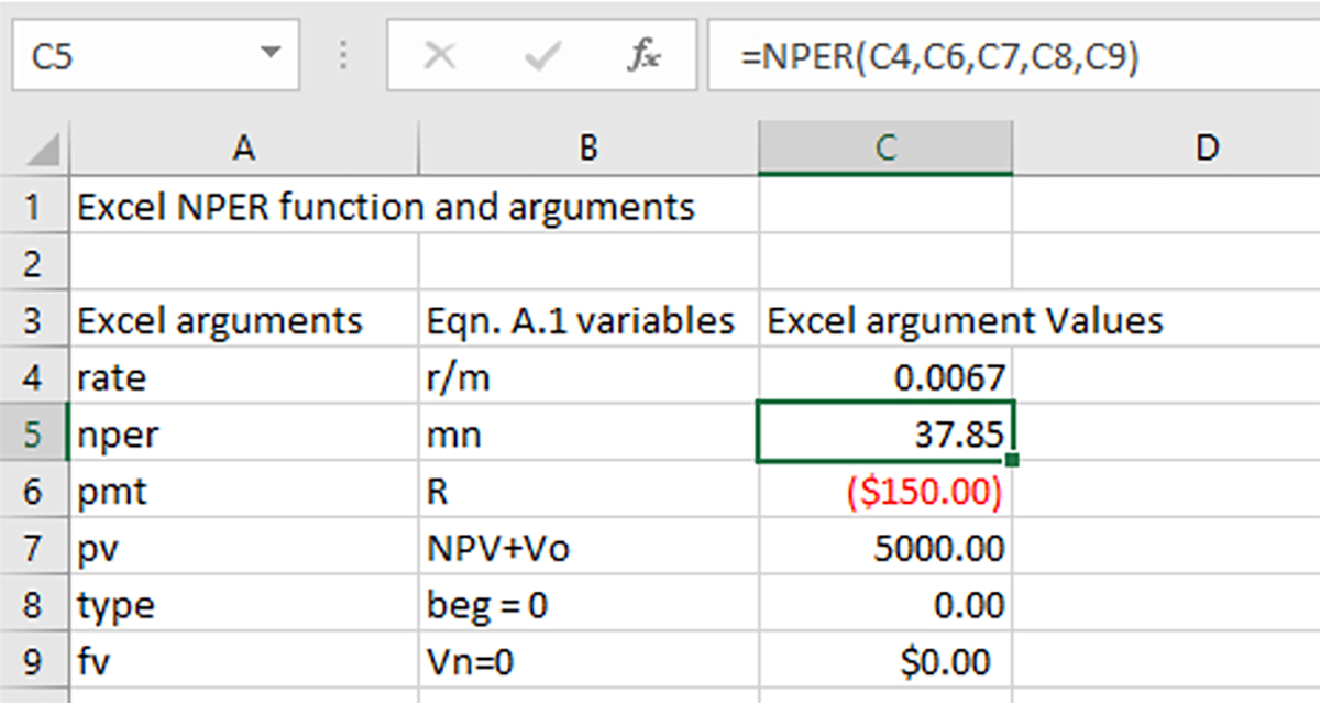
• Figure A.22. Answering the question: “what if” rate were 8%, then what would be the value of nper?
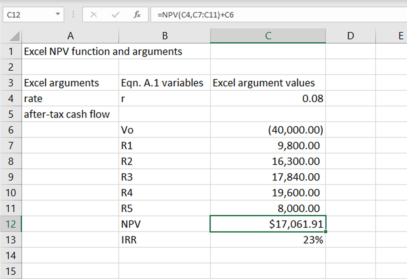
• Figure A.23. The NPV function for Green and White Services’ investment of $40,000 that produces four periods of return and then is salvaged in year 5.
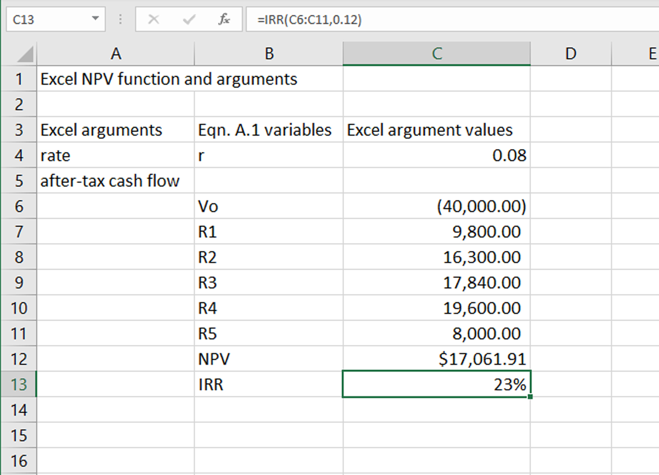
• Figure A.24. The IRR function for Green and White Services’ investment of $40,000 that produces four periods of return and then is salvaged in year 5.