Land Investments

Lindon Robison

18 Land Investments

Lindon Robison

Learning goals. After completing this chapter, you should be able to: (1) describe land’s unique investment characteristics; (2) understand how land’s endurable nature affects its price variability; (3) recognize how transaction costs reduce the liquidity of land investments; and (4) evaluate land investments using present value (PV) models developed earlier.

Learning objectives. To achieve your learning goals, you should complete the following objectives:

Learn what makes land distinct from other types of investments.
Learn why land prices are so volatile compared to other investments.
Learn how to distinguish between real and nominal discount rates.
Learn how to distinguish between inflationary and real growth in earning rates.
Learn how expected growth rates in earnings from land are capitalized into land values.
Learn how to find the real growth rate for land.
Learn how to calculate the maximum bid (minimum sell) price for land.
Learn how transaction costs associated with buying and selling land influence land’s liquidity.
Learn how taxes influence the maximum bid (minimum sell) price for land.
Learn how to find the tax adjustment coefficient for investments in land.
Learn how to use land price-to-earnings ratios to predict adjustments in the price of land.

Introduction

^[1]

Land’s immobility and durability make it unique among investments and deserving of special attention in PV analysis. Land’s immobility means that it cannot be moved and that its services must be extracted by those physically on site. Durability means that land has the capacity to provide services over time without significant change in its service provision capacity.

Earlier, an asset’s liquidity was defined as it nearness to cash. One dimension of an asset’s liquidity depends on the form of its earnings—cash versus capital gains (see Chapter 16). In this chapter we discuss a different dimension of liquidity—the cost of converting an asset to cash through its sale. Land’s immobility makes it less liquid than assets that can be moved because it cannot be moved to meet the convenience of the buyer. Land’s immobility also limits the potential buyers to those near enough to extract the land’s services. Another reason that land is illiquid is because buyers and sellers pay fees to complete its purchase and sale, including Realtor fees, legal costs of changing and recording its title, and other related fees—but not to each other. Evidence of farmland’s low liquidity is its infrequent transfer. On average, only 2% to 3% of the privately owned farmland in the United States is sold each year.

On the other hand, lenders prefer land as collateral for loans for the same reason that makes land illiquid—its immobility. Land’s immobility reduces the riskiness of it being stolen, hidden, or moved. Lenders also prefer land as collateral for loans because of its durability, which reduces the riskiness of it losing its value as security for loans. To offset some of land’s illiquidity, special institutions and programs have developed for financing residential and farm real estate.

The immobility and durability of land also make it a popular object on which to assess taxes. Taxing agencies have easy and indisputable records of the amount of land subject to tax and who owns the land. Thus, most land-owners pay property taxes on land and buildings but pay no similar tax on more mobile and less durable investments. Consequently, land is one of the few investments for which taxes are based on the market value of the investment at the beginning of the period as well as on the earnings of the investment during the period.

This chapter develops PV models to estimate maximum bid (minimum sell) prices for land investments, to describe how transaction costs contribute to land’s illiquidity, to understand how land’s durability increases its price volatility, and to demonstrate the influence of taxes on maximum bid (minimum sell) prices. We begin by describing the connection between land’s durability and its price volatility and why land and other durables are subject to inflationary bubbles and crashes.

Why are land prices so volatile?

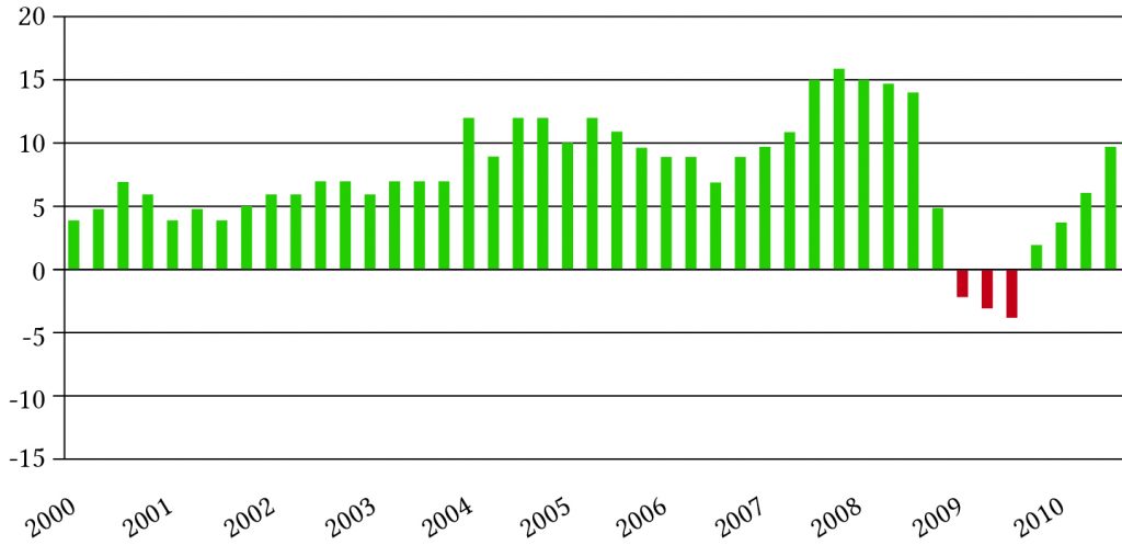
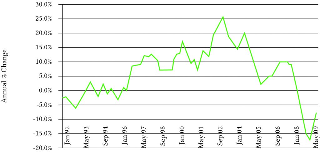
Durable price volatility. One interesting feature of farmland and other durables prices such as housing stock, is their historically high swings in values. Figure 18.1 describes year-to-year changes in Michigan farmland values over the 2000 to 2010 period. Figure 18.2 describes changes year-to-year changes in housing values over the same period. Part of these changes can be attributed to capital gains (losses). But there is another explanation for changes in the value of land and other durables, and it has to do with changes in real interest rates and real growth rates.

Graph showing year to year changes in farmland values with negative numbers only in 2009. — **Figure 18.1. Year-to-year changes in farmland values.**

Graph showing year-to-year changes in housing prices with a sharp downward turn in late 2008 through early 2009. — **Figure 18.2. Year-to-year changes in housing prices.**

Inflationary, nominal, and real interest rates. To understand price volatility of durables, it is necessary to describe inflationary, nominal, and real interest rates. Recall that the inflation rate i is equal to the rate of change in average prices, changes often linked to monetary or fiscal policies of governments. The nominal interest rate r depends on the rate of inflation and a real component that is dependent on factors other than the rate of inflation such as changing market conditions or changes in productivity. To describe the effects of inflation on the nominal interest, let one plus the nominal interest rate r equal one plus the real rate r^* times one plus the inflation rate i so that:

(18.1) $\begin{equation*} (1+r) = (1+r^*)(1+i) \end{equation*}$

We solve for the real interest rate in equation (18.1) as:

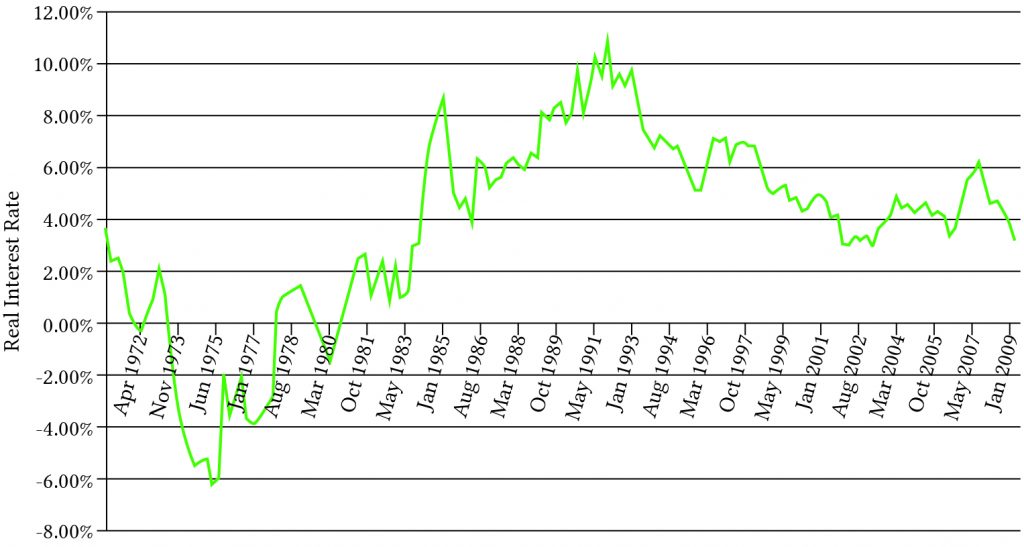
(18.2) $\begin{equation*} r^* = \dfrac{r-i}{(1+i)} \end{equation*}$

Historically, real interest rates vary by sectors but are highly correlated. Real interest rates on home loans are described graphically in Figure 18.3:

Graph showing real home loan interest rates peaking in 1985 and 1991. — **Figure 18.3. Real home loan interest rates.**

We can describe the effects of changes in the real growth rate on durable asset prices by letting the nominal growth rate g equal one plus the real growth rate g^* times one plus the inflation rate i, so that:

(18.3) $\begin{equation*} (1+g)= (1+g^*)(1+i) \end{equation*}$

We solve for the real growth rate in equation (18.3) as:

(18.4) $\begin{equation*} g^* = \dfrac{g-i}{(1+i)} \end{equation*}$

To understand the volatility of farmland prices, we build a general PV model where V₀ is land’s present value, g is the average nominal growth (decay) rate of net cash flow, r is the nominal interest rate, and R₀ represents initial cash flow. For the moment we ignore taxes and write the relationship between the variables just described in a growth model as:

(18.5) $\begin{equation*} V_0 = \dfrac{R_0(1+g)}{(1+r)} + \dfrac{R_0(1+g)^2}{(1+r)^2} + \dfrac{R_0(1+g)^3}{(1+r)^3 }+ \cdots = \dfrac{R_0(1+g)}{(r-g)} \end{equation*}$

We call the result the value in use model because there are no sales or purchases implied. Suppose we replace (1 + r) with the right-hand side of equation (18.1) and (1 + g) with the right-hand side of equation (18.3). After the substitution, we obtain the result:

(18.6) $\begin{equation*} V_0 = \dfrac{R_0(1+g^*)(1+i)}{(1+r^*)(1+i)} + \dfrac{R_0[(1+g^*)(1+i)]^2}{[(1+r^*)(1+i)]^2} + \dfrac{R_0[(1+g^*)(1+i)]^3}{[(1+r^*)(1+i)]^3}+ \cdots \end{equation*}$

Notice that the inflationary effects on the discount rate and the growth (decay) rate cancel, so that we can write equation (18.6) as a function of only real rates and initial cash flow:

(18.7) $\begin{equation*} V_0 = \dfrac{R_0(1+g^*)}{(1+r^*)} + \dfrac{R_0(1+g^*)^2}{(1+r^*)^2} + \dfrac{R_0(1+g^*)^3}{(1+r^*)^3 }+ \cdots = \dfrac{R_0(1+g^*)}{(r^* - g^*)} \end{equation*}$

Suppose that in equation (18.7), r^* changes. To measure the impact of a change in r^*, we differentiate V₀ with respect to r^* and obtain:

(18.8) $\begin{equation*} \dfrac{dV_0}{dr^*} = \dfrac{-R_0(1+g^*)}{(r^*-g^*)^2} \end{equation*}$

The percentage change in V₀, with respect to a change in r^*, equals the change in the asset’s value in response to a change in the real interest rate, equation (18.8), divided by the asset’s initial value V₀, the right-hand side of equation (18.7):

(18.9) $\begin{equation*} \dfrac{dV_0/dr^*}{V_0} = \dfrac {-1}{(r^*-g^*)} \end{equation*}$

Now suppose that g^* changes. To measure the impact of a change in g^* we differentiate V₀ with respect to g^* in equation (18.7) and obtain:

(18.10) $\begin{equation*} \dfrac{dV_0}{dg^*} = \dfrac{R_0(1+g^*)}{(r^*-g^*)^2} \end{equation*}$

The percentage change in V₀ with respect to a change in g^* equals the change in the asset’s value in response to a change in the real interest rate, equation (18.10) divided by the asset’s initial value V₀ described in equation (18.7).

The percentage change in V₀ with respect to a change in g^* equals:

(18.11) $\begin{equation*} \dfrac{dV_0/dg^*}{V_0} = \dfrac {1}{(r^*-g^*)} \end{equation*}$

We now describe the percentage changes in asset values in response to changes in the real discount rate and the real growth rate for alternative real interest rates and real capital gains (capital loss) rates. In the previous chapter we described changes in asset values over time. This analysis is different (and static or timeless). We consider what happens to an asset’s value at a point in time if one of the underlying variables that determines its value is changed.

In Table 18.1 calculations are based on equation (18.11). In the calculations we set the percentage change in asset values for alternative values of r^* and g^*. We set r^* equal to 2%, 4%, 6%, 8%, and 10%. We set g^* equal to –20%, –10%, –5%, 0%, 2% and 4%. Negative values for g^* correspond to depreciable durable assets such as buildings and machinery. Positive values of g^* are harder to justify and may reflect speculative bubbles in which asset earnings are expected to grow in real terms in perpetuity—an assumption which is hard to justify.


	g^* = –20%	g^* = –10%	g^* = –5%	g^* = 0%	g^* = 2%	g^* = 4%
r^* = 2%	–4.5%	–8.3%	–14.3%	–50%	n.a.	n.a.
r^* = 4%	–4.1%	–7.1%	–11.1%	–25%	–50%	n.a.
r^* = 6%	–3.8%	–6.3%	–9.1%	–16.7%	–25%	–50%
r^* = 8%	–3.6%	–5.6%	–7.7%	–12.5%	–16.7%	–25%
r^* = 10%	–3.3%	–5%	–6.7	–10%	–12.5%	–16.7%

Consider Table 18.1. Note that an asset’s durability is reflected by its real growth (decay) rate—an asset’s durability decreases with its g^* value. Also note that the percentage change in asset values in response to increases in real interest rates decreases with an asset’s durability. For example, if the real interest rate were 4%, a small increase in the real interest rate would cause a 4.1% decrease in the value of a depreciable asset with a negative real growth rate of –20%. Meanwhile, a small increase in the real interest rate for a durable asset with a 4% real growth rate would result in a 50% decrease in the value of an asset.

Now consider Table 18.2, which examines the effect of small increases in the real growth rate for the same scenarios described in Table 18.1 and also based on equation (18.11). The difference between Table 18.1 and Table 18.2 is that the signs within the body of the tables are reversed. An increase in the real interest rate reduces asset values because future dollars are worth less with a higher discount rate. In contrast, an increase in the real growth rates means there are more future cash flows to discount—making the change in the value of the assets positive in response to a small increase in the real growth rate.

Table 18.2. Percentage changes in asset values corresponding to 1% changes in real growth rate for alternative values of r^*and for assets with various degrees of durability characterized by the variable g^*.
	g^* = –20%	g^* = –10%	g^* = –5%	g^* = 0%	g^* = 2%	g^* = 4%
r^* = 2%	4.5%	8.3%	14.3%	50%	n.a.	n.a.
r^* = 4%	4.1%	7.1%	11.1%	25%	50%	n.a.
r^* = 6%	3.8%	6.3%	9.1%	16.7%	25%	50%
r^* = 8%	3.6%	5.6%	7.7%	12.5%	16.7%	25%
r^* = 10%	3.3%	5%	6.7	10%	12.5%	16.7%

One interesting feature of Table 18.2 is that the percentage change in asset values in response to small increases in the real growth rate are dampened by higher real interest rates. For that reason, when the economy is “overheated” and prices are rising, one response is to reduce the money supply, increasing the real interest rate and slowing price increases. For example, suppose the real growth rate were zero% and the real interest rate was 2%. If the real growth rate increased slightly, the asset value would increase by 50%. If, instead, the real interest rate were 10% and the real growth rate increased slightly, the asset value would increase by only 10%.

So, what have we learned? We learned that durable assets such as land and houses are subject to significant percentage changes in value in response to changes in real interest rates and real growth rates—much more so than depreciable assets. In addition, changes in the asset’s real growth rate in earnings have less effect when real interest rates are high.

To test your understanding of the material just covered, demonstrate that a 1% increase in the real growth rate produces the same percentage changes in asset values as those described in Table 18.1, except opposite in sign.

Maximum Bid (Minimum Sell) Price Models and Transaction Costs

Maximum bid (minimum sell) price models. We now deduce maximum bid price models for buyers and minimum sell price models for sellers. At least two costs differentiate maximum bid price models for buyers and minimum sell price models for sellers: taxes and transactions costs. Let c equal the percentage of land’s sale price paid by the buyer to purchase the land—but not paid to the seller. These may include loan closing fees, title examination and registration fees, attorney’s costs, and closing points paid by the buyer. Let s equal the percentage of the land’s sale price paid by the seller to sell the land—but not paid to the buyer. This may include loan closing fees, Realtor fees, advertising, and other fees.

Denote V₀^b as the buyer’s maximum bid price and V₀^s as the seller’s minimum sell price. Ignoring taxes, and assuming that the land will never be sold again, the expression for V₀^b can be written as:

(18.12) $\begin{equation*} (1+c)V_0^b = \dfrac{R_0(1+g)}{(1+r)} + \dfrac{R_0(1+g)^2}{(1+r)^2} + \dfrac{R_0(1+g)^3}{(1+r)^3 }+ \cdots = \dfrac{R_0(1+g)}{(r-g)} \end{equation*}$

Expression (1 + c)V₀^b represents the maximum bid price, including the effect of closing costs. To isolate the maximum bid price, we solve for V₀^b.

(18.13) $\begin{equation*} V_0^b = \dfrac{R_0(1+g)}{(r-g)(1+c)} \end{equation*}$

In the maximum bid price model, the discounted stream of future cash flow represents the challenging investment—the present value of earnings the buyer will receive if the land is purchased.

Example 18.1: Finding the Maximum Bid Price for Land. What is the maximum bid price of a parcel of land if the buyer pays 6% of the acquisition price as a closing fee? To solve the problem, assume last year’s net cash flow was $22,000, which is expected to grow in perpetuity at 4.5%. Assume that the buyer’s opportunity cost of capital is 12%. The maximum bid price is calculated using equation (18.13):

(18.14) $\begin{equation*} V_0^b = \dfrac{R_0(1+g)}{(r-g)(1+c)} = \dfrac {\$22,000(1.045)}{(.12-.045)(1.06)} = \$289,182 \end{equation*}$

If closing costs, as a percentage of the price, increase from 6% to 9%, V₀^b decreases to $281,223.

Minimum sell price models. Realtor fees and other closing costs paid by the seller are now introduced into the minimum sell price model. To build the minimum sell price model, let sV₀^s be subtracted from the seller’s proceeds. Ignoring taxes and assuming that the land will only be sold one time, we can write the minimum sell price model as:

(18.15) $\begin{equation*} (1-s)V_0^s = \dfrac{R_0(1+g)}{(1+r)} + \dfrac{R_0(1+g)^2}{(1+r)^2} + \dfrac{R_0(1+g)^3}{(1+r)^3 }+ \cdots = \dfrac{R_0(1+g)}{(r-g)} \end{equation*}$

Solving for V₀^s, we find the minimum sell price equal to:

(18.16) $\begin{equation*} V_0^s = \dfrac{R_0(1+g)}{(r-g)(1 - s)} \end{equation*}$

In the minimum sell price model, the discounted stream of future cash flow represents the defending investment—it represents the earnings the seller would not earn if the land were sold.

Example 18.2: Finding the Minimum Sell Price. Letting s = 2% and using the data from Example 18.1, we find the minimum sell price using equation (18.13):

(18.17) $\begin{equation*} V_0^s = \dfrac{R_0(1+g)}{(r-g)(1 - s)} = \dfrac {\$22,000(1.045)}{(.12-.045)(.98)} = \$312,789 \end{equation*}$

Now, suppose s increases from 2% to 3%. In turn, V₀^s increases to $316,014. In contrast to the effects of an increase in c that reduced the maximum bid price, an increase in s increases the minimum sell price:

Land Values, Transaction Costs, and Liquidity

Suppose a buyer and a seller had the same earnings expectations and opportunity costs for a durable such as farmland. It must follow that their present-value for the durable in use would be the same. But if the buyer had to pay closing fees to acquire the durable, his maximum bid price would be reduced. And if the seller received only a portion of the present value after the sale, her minimum sell price would increase. Therefore, transaction costs that increase the seller’s minimum sell price and reduce the buyer’s maximum bid price reduce the liquidity of the durable, even when the buyer and seller have the same earnings expectations and opportunity costs.

In other words, an asset is illiquid if its value in use (V₀) is bounded below by a buyer’s maximum bid price (V₀^b) and bounded above by the seller’s minimum sell price (V₀^s). We can easily show that assets for individuals with identical expectations of land’s value in use are illiquid when transaction costs are imposed on its sale and purchase.

Substitute the value in use from equation (18.5) into the maximum bid price model in equation (18.13), and the result is:

(18.18) $\begin{equation*} V_0^b = \dfrac{R_0(1+g)}{(r-g)(1+c)} = \dfrac{V_0}{(1+c)} < V_0 \end{equation*}$

It should be clear that for c > 0, V₀^b < V₀.

Next, substitute the value in use from equation (18.5) into the minimum sell price model in equation (18.16) and the result is:

(18.19) $\begin{equation*} V_0^s = \dfrac{R_0(1+g)}{(r-g)(1-s)} = \dfrac{V_0}{(1-s)} > V_0 \end{equation*}$

It should be clear that for s > 0, V₀ < V₀^s. Finally combining these results allows us to express the effects of transaction costs on the maximum bid, minimum sell, and value-in-use models:

(18.20) $\begin{equation*} V_0^b < V_0 < V_0^s \end{equation*}$

Despite equal earning expectations, as a result of transaction costs, the maximum bid price is less than the minimum sell price making land illiquid. To make this point another way, suppose that we formed the ratio of the maximum bid price and the minimum sell price for land and assumed that c = 5% and s = 6%. Then the buyer in this example would only be willing to offer 89.2% of the seller’s minimum sell price, and a sale would not occur.

(18.21) $\begin{equation*} \dfrac{V_0^b}{V_0^s} = \dfrac{(1-s)}{(1+c)} = \dfrac{1-.06}{1+.05} = 89.2\% \end{equation*}$

Other Factors Contributing to Asset Liquidity

Differences in financing costs for buyers and sellers may also contribute to an asset’s illiquidity. For example, a loan tied to the ownership of durables at below-market interest rates may create a wedge between the maximum bid price and the minimum sell price. If the loan has a due-on-sale clause, the seller gives up something of value that is not received by the buyer when the investment is sold. Thus, concessionary interest rate loans with due-on-sale clauses may create illiquidity.

Differences in information between the buyer and seller may also contribute to an asset’s illiquidity. When two trusted friends exchange a durable, the information costs are insignificant—they freely exchange information. However, when two strangers exchange a durable, the buyer must commit resources to discover the quality of the information provided by the seller. If an investment’s service capacity is easily observed, as with certified seed or fertilizer, then the information cost is small and the investment will be more liquid. Durables like used cars or tractors, whose remaining service capacity is not easily observed, will be less liquid. The issuance of a warranty is a signal of higher quality, and thus a warranty is an attempt to reduce information costs for the prospective buyer and to increase the liquidity of the asset.

The cost of gathering information about the asset’s service capacity may also contribute to its liquidity. To illustrate, a new asset’s service capacity may be well known. Once the durable is used, however, the uncertainty associated with the intensity of use and care of the durable creates an immediate decline in the value of the durable. On the other hand, a used durable whose service extraction is nearly depleted is more liquid, because there is nearly perfect information about the durable’s remaining capacity.

The liquidity of durables is also affected by disposal costs. Disposal cost is the cost of removing durables from service paid by its current owner. Most durables are mobile. Buildings, however, must be disassembled at considerable costs. In some cases, the investment is so valuable that assembly and disassembly are warranted. An example is the London Bridge. Most durables with high disposal costs become completely illiquid and remain in service to the first owner until destroyed. Often it is easier to transfer the owner rather than the investment itself. Examples of durables with high disposal costs are land and houses.

Durables whose value increases with time and use are called appreciating durables. Durables whose values decrease with time and use are called depreciating durables. A durable whose value increases with time and use will be more liquid than one whose value declines with time and use, with all other liquidity attributes held constant. Appreciating durables provide greater security for lenders than depreciating durables because their value and the lender’s security are increasing. Finally, liquidity is affected by whether or not time or use determines the durables’ service capacity. Durables whose service capacity is determined by time have a fixed pattern of changes in service capacity and cannot adjust to changes in the market. Durables whose change in service capacity is determined by use can adjust to changes in the marketplace for the value of its services. Thus, durables whose service capacity is tied to use are more liquid than those whose service capacity is linked to time.

The liquidity of a durable is also influenced by the number of services the durable can provide. Durables become more liquid if the buyer has opportunities for the durables’ services that are not available to the seller. A durable is more likely to have multiple uses when it is not fixed geographically. Multiple use capability is also tied to the acquisition characteristics of the durable. If the durable is lumpy in acquisition, potential buyers must take it or leave it. Durables divisible in acquisition, on the other hand, provide options for prospective buyers. They can buy a gallon or a tankful of gas, a sack of seeds or a truckload.

Finally, durables whose service extraction rate is fixed, and hence irreversible, are less liquid than durables whose service extraction rate is variable. Variations in service capacity provide greater adjustment potentials, and thus reduce the differences in perceptions between buyers and sellers. Moreover, durables whose service extraction rates vary tend to have multiple uses, while those with fixed service extraction rates tend to be single-use durables.

Maximum Bid (Minimum Sell) Land Price Models with Taxes

Taxes are now introduced into our maximum bid (minimum sell) price for land models. As mentioned earlier, land is subject to a wide variety of taxes, not all of which are imposed on other assets. Four kinds of taxes must be considered in our maximum bid (minimum sell) price for land models: First, the cash flow stream is taxed at the average income tax rate T. Second, the opportunity cost of capital r is expressed on an after-tax basis. Since the discount rate may reflect the opportunity cost of capital associated with investments that earn both capital gains and cash, the tax rate is θT. Third, property taxes (T_p) are another tax charged against the market price of land in each period. Thus, land’s maximum bid price in future periods must be included in each period. The study of capital gains indicated that land prices should increase at the same rate as land earnings. Finally, one tax not included in the land price models is tax-savings rate T_g, resulting from durable depreciation. The reason is simple—land is not considered a depreciable investment.

The Maximum Bid Price Model with Taxes. The expanded maximum bid price model with taxes is written as:

(18.22) $\begin{equation*} \begin{split} (1+c)V_0^b & = \dfrac {R_0(1+g)(1-T)-V_0^b T_p(1-T)} {[1+r(1- \theta T)]} \\ & + \dfrac {R_0(1+g)^2(1-T)-V_0^b (1+g)T_p(1-T)} {[1+r(1- \theta T)]^2} + \cdots = S_1 + S_2 \end{split} \end{equation*}$

The cash flow stream contains two geometric series. In both series, the geometric factor is (1 + g)/ [1 + r(1 – θT)] and the sums of the two series are equal to:

(18.23) $\begin{equation*} \begin{split} S_1 & = \dfrac {R_0(1+g)(1-T)} {[1+r(1- \theta T)]} + \dfrac {R_0(1+g)^2(1-T)} {[1+r(1- \theta T)]^2} + \cdots \\ & = \dfrac {R_0(1 + g)(1 - T)}{r(1- \theta T)-g} \end{split} \end{equation*}$

while

(18.24) $\begin{equation*} \begin{split} S_2 & = - \dfrac{V_0^b T_p(1-T)}{[1+r(1- \theta T)]} - \dfrac{V_0^b (1+g) T_p(1-T)}{[1+r(1- \theta T)]^2} - \cdots \\ & = - \dfrac{V_0^b T_p(1-T)}{r(1- \theta T)-g} \end{split} \end{equation*}$

Finally, setting (1 + c)V₀^b equal to the sum of S₁ and S₂ and solving for V₀^b, the maximum bid price with taxes of land can be written as:

(18.25) $\begin{equation*} V_0^b = \dfrac{R_0(1+g)(1-T)}{[r(1- \theta T)-g](1+c)+T_p(1-T)} \end{equation*}$

It is still the case that the challenging investment in equation (18.16) is represented by the discounted after-tax cash flow stream while the defender is the maximum bid price plus closing fees, which earns the discount rate r given up to acquire the income earning durable.

Example 18.3: Maximum Bid Price with Taxes. An investor is interested in buying a crop farm. According to the financial statements, last year the farm generated a net cash receipts of $48,000. Past data indicated that net cash returns have been growing at 6% per year. The investor’s opportunity cost of capital is 11%, and closing fees for the transaction are 3%. The investor’s income tax bracket is 30%, the property tax is 2%, and we assume that θ = .75. Using equation (18.25), the maximum bid price for the farm is

(18.26) $\begin{equation*} \begin{split} V_0^b & = \dfrac {\$48,000(1.06)(1-.3)}{ \left\{.11[1-(.75)(.3)] - .06\right\}(1+.03) +.02(1-.3)} = \dfrac{\$35,616}{.026+.014} \\ & = \$890,400 \end{split} \end{equation*}$

The Value in Use model. It will be convenient later on to find the value of what the seller will sacrifice instead of selling his or her land and continuing to extract services from it. In this case there are no transaction costs, and property taxes are associated with its use value as opposed to its maximum bid price. We can derive the value in use with taxes model, V₀^u, by setting c = 0 in equation (18.25). The result is:

(18.27) $\begin{equation*} V_0^u = \dfrac{R_0(1+g)(1-T)}{[r(1- \theta T)-g] + T_p(1-T)} \end{equation*}$

To illustrate, the value in use model for the previous example is:

(18.28) $\begin{equation*} V_0^u = \dfrac{\$48,000(1.06)(1-.3)}{\left\{.11[1-(.75)(.3)]-.06\right\} +.02(1-.3)} = \$913,230 \end{equation*}$

One way to interpret the value in use with taxes model is that it represents the defending asset for the seller of land—the present value of future earnings it would receive, provided the land isn’t sold.

The Minimum Sell Price Model with Taxes. The minimum sell price model with taxes is similar to the maximum bid price model with taxes, with a few exceptions: First, assume the seller originally bought his or her land t periods earlier at a price of V_-t^b. Then, if V_-t^b is less than (more than) the current selling price of V₀^s, the seller pays (earns) capital gains taxes (credits) at a rate of α times the average income tax rate of αT% or αT.

Another difference is the transaction costs. These costs affect taxable capital gains because the capital gains tax is only paid on the net gain from the sale of land. Like the maximum bid price model, however, the property tax rate is assessed against the inflating value in use since there is no benchmark sell price to calibrate its tax value.

The value in use with taxes is the challenging investment for the seller. We equate the after-tax sale price to the value in use with taxes in equation (18.29). We summarize these results in equation (18.29):

(18.29) $\begin{equation*} \begin{split} (1-s)V_0^s & - [(1-s)V_0^s - (1+c)V_{-t}^b \alpha T \\ & = V_0^u = \dfrac{R_0(1+g)(1-T)}{[r(1- \theta T)-g] + T_p(1-T)} \end{split} \end{equation*}$

Solving for V₀^s the minimum sell price with taxes we find:

(18.30) $\begin{equation*} V_0^s= \dfrac {V_0^u - (1+c)V_{-t}^b \alpha T}{(1-s)(1 - \alpha T)} \end{equation*}$

Example 18.4: Minimum Sell Price with Taxes. ABC Corporation wants to sell a large farm. They want to know their minimum sell price to accept—or the price a buyer would need to offer in order for them to be as well off selling as they would be continuing to farm the land. ABC has already calculated the farmland’s value in use is equal to $913,230 (see equation 18.27). This is the present value of their defender.

Recognizing its minimum sell price adjusted for transaction costs and capital gains taxes (credits) as its challenger, ABC equates the two, and solves for its minimum sell price with taxes. The result is expressed in equation (18.30). Summarizing the information needed to find ABC’s minimum sell price: V₀^u = $913,230, c = 3%, V_-t^b = $600,000, α = .4, T = 30%, and s = 5%.

The result is:

(18.31) $\begin{equation*} \begin{split} V_0^s & = \dfrac {V_0^u - (1+c)V_{-t}^b \alpha T}{(1-s)(1 - \alpha T)} = \dfrac {\$913,230 - (1.03)(\$600,000)(.4)(.3)}{(.95)[1-(.4)(.3)]}\\ & = \$1,003,672 \end{split} \end{equation*}$

Clearly, the buyer and seller in Examples 18.3 and 18.4 would never exchange land—the minimum sell price of $1,003,672 exceeds the buyer’s maximum bid price of $890,400. What would have to change for land to become liquid—for the buyer to offer the seller at least his or her minimum sell price? Well, for one thing, the buyer would have to expect initial earnings greater than $48,000. Or the buyer could find means of reducing its property tax rate. Or the buyer could reduce its transaction costs. Or the buyer may have a lower opportunity cost than the seller. Other changes, such as changes in g and T, have ambiguous effects on the maximum bid price V₀^b.

Finding the Tax Adjustment Coefficient θ

The homogeneity of measures principle requires that after-tax cash flow be discounted by an after-tax discount rate—in most cases the IRR of the defender. The question is, how do we find the after-tax IRR that corresponds to the after-tax cash flow of the defender? First, we specify the defender’s cash flow stream and PV and solve for the discount rate or the IRR of the investment. We are guaranteed that we have found the IRR of the defender in a maximum bid (minimum sell) price model and value in use model because the NPV in these models is always zero. We demonstrate how to find the defender’s IRR first for the simple geometric growth model and then for more complicated models that include taxes.

Now we introduce taxes into equation (18.5), holding V₀ constant, and express the after-tax geometric growth model as:

(18.32) $\begin{equation*} \begin{split} V_0 & = \dfrac{R_0(1+g)(1-T)}{[1+ r(1- \theta T)]} + \dfrac{R_0(1+g)^2(1-T)}{[1+ r(1- \theta T)]^2} + \dfrac{R_0(1+g)^3(1-T)}{[1+ r(1- \theta T)]^3} + \cdots \\ & = \dfrac{R_0(1+g)(1-T)}{r(1- \theta T)-g}\end{split} \end{equation*}$

To summarize, because equation (18.32) describes a defender’s after-tax cash flow stream, then r(1 – θT) is the defender’s after-tax IRR—because NPV in equation (18.32) is zero. Another way to summarize the results above is to note that taxes in equation (18.32) are neutral—meaning that they are introduced so that NPV remains zero. Since V₀ is the same in both equations (18.5) and (18.32), we can equate their right-hand sides and write:

(18.33) $\begin{equation*} V_0 = \dfrac{R_0(1+g)(1-T)}{r(1- \theta T) -g} = \dfrac{R_0(1+g)}{(r-g)} \end{equation*}$

Up to this point, we have not specified the value of θ. However, we do require that its value be chosen in such a way that r(1 – θT) is the after-tax IRR of the defender’s after tax cash described using a geometric growth model. We find such a θ for the geometric cash flow model using equation (18.32), which equals:

(18.34) $\begin{equation*} \theta = \dfrac{r-g}{r} \end{equation*}$

The above results are intuitive. For g ≠ 0 in equation (18.34), capital gains (losses) are earned (lost) without creating any tax consequences. If the before-tax IRR is r, an after-tax rate of r(1 – T) implies cash and capital gains (losses) are taxed at the average income tax rate T, which is not true because only cash receipts are taxed. Since capital gains (losses) are earned (lost) at rate g, subtracting from r%, g%, makes taxes neutral in the geometric growth model described above. To confirm that θ coefficient makes taxes neutral, the right-hand side of equation (18.34) is substituted into equation (18.33) to obtain the result:

(18.35) $\begin{equation*} V_0 = \dfrac {R_0(1+g)(1-T)}{ \left\{ r \left[ 1 - \left(\dfrac{r-g}{r}\right) T \right] - g \right\}} = \dfrac{R_0(1+g)}{(r-g)} \end{equation*}$

Following a similar procedure, we can find the value for θ in the value in use model for land. In this case, we equate the right-hand side of the value in use land model to the right hand side of the geometric growth model. This new equality can be written as:

(18.36) $\begin{equation*} V_0^u = \dfrac{R_0(1+g)(1-T)}{[r(1- \theta T)-g] + T_p(1-T)} = \dfrac{R_0(1+g)}{r-g} \end{equation*}$

As before, θ in equation (18.36) is the coefficient that makes taxes neutral in the land value in use model because it ensures that the effects of taxes on the defender’s cash flow are equally offset by changes in the discount rate. Therefore, the discount rate continues to equal the defender’s IRR. We can find such a θ for a value in use land model by solving for θ in equation (18.36):

(18.37) $\begin{equation*} \theta = \dfrac{r-g +(T_p/T)(1-T)}{r} \end{equation*}$

Clearly, property taxes increase the tax adjustment coefficient and the effective tax rate.

Non-neutral taxes. When we calculated the tax-adjustment coefficient, we assumed tax-neutrality. This was an appropriate assumption for finding the after-tax IRR of the defender. In other PV models, there is no reason to assume that the after-tax IRR of the defender used to calculate the maximum bid (minimum sell) price or NPV will be tax-neutral. For example, assume the challenger’s cash flow is represented by a geometric growth equation and assume that the tax adjustment coefficient of the defender is one—an assumption consistent with a defender’s whose returns are only cash. In this case, we find the value in use as:

(18.38) $\begin{equation*} \begin{split} V_0 & = \dfrac{R_0(1+g)(1-T)}{[1 + r(1-T)]} + \dfrac{R_0(1+g)^2(1-T)}{[1 + r(1-T)]^2} + \cdots \\ & = \dfrac{R_0(1+g)(1-T)}{ r(1-T)-g} \end{split} \end{equation*}$

To test for tax-neutrality, we differentiate V₀ with respect to T and find:

(18.39) $\begin{equation*} \dfrac{dV_0}{dT} = \dfrac{gR_0(1+g)}{[r(1-T)-g]^2} > 0 \end{equation*}$

In this particular case, taxes are not neutral, and increasing the tax rate makes the defender less attractive relative to the challenger because the challenger’s capital gains are shielded from income taxes.

Price-to-earnings Ratios for Land

An interesting ratio can be derived from the value in use with taxes model, equation (18.32). It is the ratio of land’s value in use, divided by the previous period’s cash flow, approximated by cash rents. We write the ratio as:

(18.40) $\begin{equation*} \dfrac{V_0}{R_0} = \dfrac{(1+g)(1-T)}{[r(1-T)-g] + T_p(1-T)} \end{equation*}$

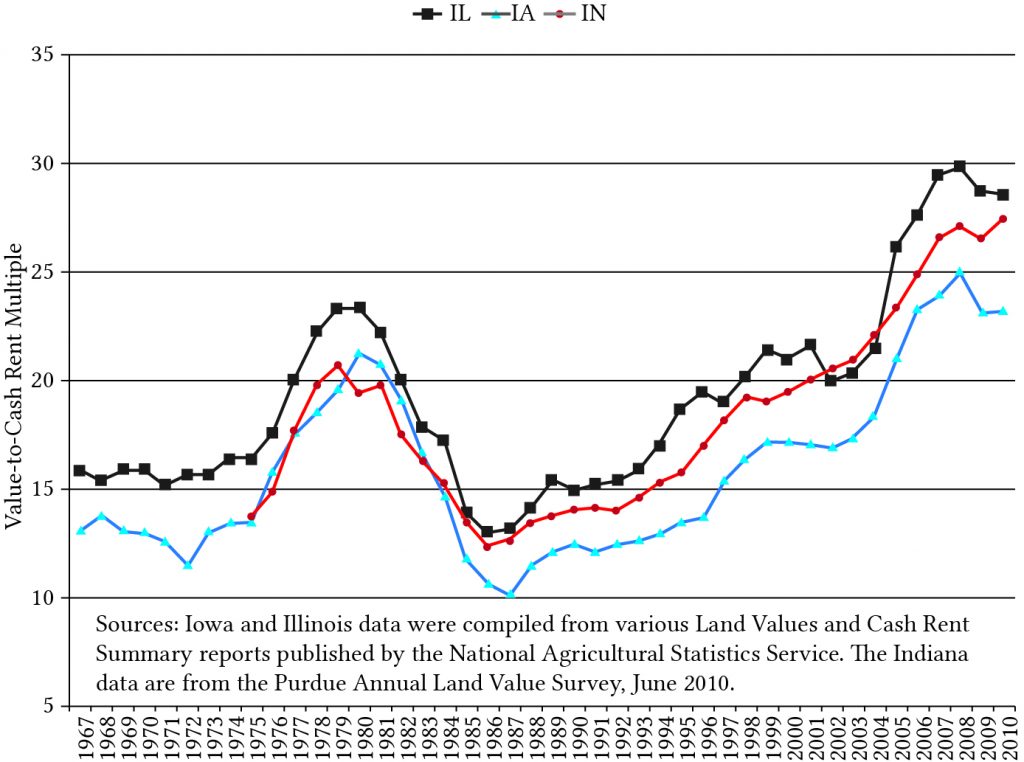
Note that the value-to-earnings ratio for land depends on specific tax rates, opportunity costs, and expected growth rates, and these vary from location to location. Figure 18.4 below describes land values to rent ratios for land in Iowa, Illinois, and Indiana since 1967. Suppose that in equation (18.40) we were to ignore taxes and assume a real growth rate of zero. Then equation (18.40) reduces to the traditional capitalization ratio of:

(18.41) $\begin{equation*} \dfrac{V_0}{R_0} = \dfrac{1}{r^*} \end{equation*}$

This is how the traditional capitalization ratio is derived. As an earlier graph demonstrated, however, the ratio has not been constant over time.

Graph showing land values to rent ratios for land in Iowa, Illinois, and Indiana since 1967. The ratio of land to rent values increased through the 1970s, decreased through the early 1980s, and then increased since 1987. — **Figure 18.4. Land values to rent ratios for land in Iowa, Illinois, and Indiana since 1967.**

An interesting exercise would be to approximate the discount rate in equation (18.41) with the real interest rate described in an earlier figure and then compare the results with the ratios described above.

Summary and Conclusions

Land’s immobility and durability make it an important asset for securing loans. Its immobility means that lenders know where to find it, and its durability means that it will have the capacity to supply services and earn a return almost undiminished into the future. Both of these characteristics provide assurances to lenders that if they loan money to buy land, they will be able to recover their loans even if the borrowers fail to meet their obligations. On the other hand, land’s immobility and durability also mean that its owners’ can be easily identified and taxed. Land sales are carefully recorded to establish its value. Thus, land is a favorite source of tax revenue not only for its market value but also at the time of sale if capital gains (losses) are incurred.

Land has another feature. Land is infrequently traded, and transfers of ownership are costly for both buyers and sellers—often requiring the help of outside agents who must be paid for their services. As a result, both buyers and sellers pay funds they do not receive when buying and selling land. These transaction costs, including tax payments, mean that land exchange will likely not occur unless the buyer expects to earn more from land’s services than currently earned by sellers. As a result, land is illiquid and its purchase and sale is a very infrequent occurrence.

In this chapter, PV models were used to model three types of prices: maximum bid prices, the most a buyer could offer to purchase the land; minimum sell prices, the least a seller would accept to sell the land; and value in use prices, the value of the land assuming continued use. These models accounted for three different types of taxes (property tax, income tax, and capital gains tax) as well as cash flow. These models provide helpful tools for assisting buyers and sellers in determining investment strategies.

Questions

Describe the features that make land an illiquid investment.
Why do lenders seem to prefer land to secure their loans? Compare the loan security provided by land compared to that offered by used equipment or breeding livestock?
Figures 18.1 and 18.2 compare year-to-year changes in farmland and housing prices. What is similar between those forces contributing to the variability in the prices of land and housing stock?
Commodities are nondurable goods and are likely used up in a single period. Meanwhile, land and houses are durables and last for many years. Can you describe how these differences between durable and nondurable goods may contribute to differences in the variability of their prices? Does the fact that the supply of land is relatively fixed versus the supply of commodities that can vary from year to year influence their variability?
Equation (18.9) describes the percentage change in the price of a long term asset (in this case land) in response to a change in the real interest rate r^*. Assume that the real growth rate is 3% and the real interest rate is 4%. Find the percentage increase in V₀ if r^* increases by 1%. Find the percentage increase in V₀ if g^* decreases by 1%.
Consider the maximum bid price and minimum sell price models. Consider the following data: the closing fee for the buyer is 3%, the closing fee for the seller is 4%, and in the last period land rented for $150 per period. Land is liquid if the maximum bid price is greater than the minimum sell price. Using this data, please answer the following questions. Calculate the ratio of the maximum bid price to the minimum sell price. Is land liquid or illiquid? What must occur for the land to become liquid?
An investor is interested in buying a crop farm. According to the financial statements last year, the farm generated a net cash flow of $52,000. Past data indicates that net cash returns have been growing at 3% per year. The investor’s opportunity cost of capital, the IRR on its defender, is 8%, and closing fees for the transaction are 4%. The property is taxed at 1.5%, and the investor is in the 35% tax bracket. The tax adjustment coefficient θ is assumed to equal 75%. Find the maximum bid price for the parcel of land using maximum bid price with taxes model.
Farmland owners Rob and Ruthie Bell want to retire and sell their farm. They purchased their farm over 30 years ago for $325,000. They recognize that their minimum sell price must leave them as well off as they would be if they continued to operate their farm. They estimate that closing fees will equal 3%, they are in the 30% tax bracket, and their capital gain tax rate αT is 12%. Finally, they realize that their closing fees will be 5%. Find the minimum sell price for Rob and Ruthie Bell. (Hint: first find the value in use with taxes for the farmland. Then using the value in use with taxes and data described in this question, calculate the minimum sell price using the minimum sell price with taxes model.)
In previous problems, the tax adjustment coefficient was assumed to be 75%. Using the data supplied for calculating the maximum bid price for land with taxes, find the tax adjustment coefficient using equation (18.37).
Use equation (18.41) and land value to cash rent data described in Figure 18.4 to approximate real interest rates over time for Iowa, Indiana, or Illinois. If you believe that real interest rates are constant, what other explanations can you offer for time varying land value to rent ratios?

Some of the material in this chapter was adapted from Robison, L.J. and P.J. Barry (1996); Present Value Models and Investment Analysis. “Chapter 14: Transaction Costs and Land Purchase/Sale Decision”. MSU Press, East Lansing, Michigan. ↵

License

Icon for the Creative Commons Attribution-NonCommercial 4.0 International License

Financial Management for Small Businesses, 2nd OER Edition Copyright © 2021 by Lindon Robison is licensed under a Creative Commons Attribution-NonCommercial 4.0 International License, except where otherwise noted.