
9 Present Value Models
Lindon Robison
Learning goals. At the end of this chapter, you should be able to: (1) organize present value (PV) models by the questions they answer; (2) organize PV models by their unknown endogenous variables; and (3) solve practical PV problems using appropriate PV models.
Learning objectives. To reach your learning goals, you should complete the following objectives:
- Distinguish between different kinds of PV models including:
- net present value (NPV),
- internal rate of return (IRR),
- maximum (minimum) bid (sell),
- annuity equivalent (AE),
- loan formula,
- optimal term,
- replacement,
- incremental,
- capitalized value,
- break-even,
- payback.
- Describe the unknown endogenous variable that defines PV models.
- Describe the kinds of questions different PV models can answer.
- Use Excel financial formulas to solve the different kinds of PV models described in this chapter.
Introduction
Earlier we defined a PV model as a multi-period extension of an accrual income statement (AIS) that values future cash flow as though they were received in the present. Just as AISs find different earnings and rates of return measures, different PV models find different earnings and rates of return measures—and more. In addition, each type of PV model is designed to answer different kinds of questions.
Kinds of PV Models
Comparative advantage. Picture yourself traveling across the country driving a luxury car or a tractor. Alternatively, picture yourself pulling a plow with a luxury car or a tractor. While both a luxury car and a tractor can provide transportation and pulling services, they are not equally suited for the two assignments.
Economists use the words comparative advantage to describe activities a firm can perform but with unequal efficiency. Luxury cars are perfectly suited for traveling across country but not for pulling a plow. A tractor is well designed for pulling a plow but not for long-distance travel.
Similarly, there are several different kinds of PV models. Each model has a comparative advantage for answering different questions. In what follows we examine some of the most important PV models and the questions they can be used to answer.
The distinction between PV models. PV models are single equation models especially designed to find one unknown variable. Different kinds of PV models distinguish themselves from each other by the one unknown variable they are designed to find. The questions we wish to answer determine which PV model and unknown variable we wish to find. In what follows we identify and discuss the following PV models: NPV, IRR, maximum (minimum) bid (sell), annuity equivalent (AE), break-even, optimal life and replacement, and payback. We also describe the question each one is designed to answer. We emphasize that each PV model solves for one unknown variable that identifies the PV model type.
Net Present Value Models
NPV models solve for the difference between the present value of the challenger and the defender’s earnings. These earnings differences can be positive or negative. Positive (negative) NPV earnings support the conclusion that the challenging (defending) investment earns more in present value dollars than does the defender (challenger). Comparisons of more than one challenger against the same defender must calculate the challengers’ NPVs and compare them.
The important difference between NPV models and AIS profit calculations is that AIS calculations may include non-cash returns and expenses such as increases in inventory and depreciation. The numbers that enter NPV models besides the discount rate and the exponents on the discount rate are cash flow. The exception is the liquidation value of the investment at the end of its economic life that is treated as though it were converted to cash.
An illustration of an NPV calculation. Suppose an investment in a challenger requires an outflow of V0 dollars and generates a positive cash flow of R1 dollars one period later plus the investment’s liquidation value S1. For now, assume that the exchange rate between present defender dollars and future challenger dollars is r percent and represents the opportunity cost of sacrificing the defender to invest in the challenger. To determine if the benefits of the challenger outweigh the opportunity costs of disinvesting in the defender, we find the NPV defined as:
(9.1) 
Suppose a challenging investment costs $100 and returns R1 = $100 and S1 = $20 in period one while the defending investment earns r equal to 10%. Then the NPV of this investment would be:
(9.2) 
For this investment, NPV is positive, and present profits from the challenger outweigh the present loss in profits from sacrificing the defender. Another way to describe this result is that the challenger earned a higher rate of return than the defender. How much more? The exchange rate for the challenger is ($100 + $20)/$100 = 1.20 compared to $110/$100 = 1.10 for the defender.
But what does it mean to say that the challenger earned a higher rate of return than the defender? An investment is a commitment one makes to a project. If the project pays more than the rate of return on the defender, then the investment’s NPV is positive. In our example the project pays at the rate of 20%. In NPV models, think of the discount rate as the rate earned by the defending investment. And if NPV is positive, the challenger will earn a rate of return higher than could be earned by continuing to invest in the defender.
Of course, investments can be much more complicated than described above. For example, an investment may generate (positive and negative) cash flows for n periods (R1, R2, ⋯, Rn) rather than just one period. Furthermore, most capital assets generate a positive or negative liquidation value (Sn) at the end of its economic life which should be accounted for explicitly.
An Excel template solution. Suppose a firm can invest V0 = $1,000 present dollars in exchange for three future period dollars R1 = $200, R2 = $250, R3 = $350, and salvage value V3 = $950. Also assume that the defender exchanges dollars between time period at the rate of (1.08). Excel finds the NPV of the investment just described using its NPV equation described below in Table 9.1 equal to $431.50. To make the Excel solution transparent, the function fx= NPV(B1,B3:B4,(B5+B6))–B2 describes the cell location of the variables included in the solution. Meanwhile, an explanatory equation containing variable names is listed to the right of the NPV equation, =PV(r,V0,R1,R2,R3+V3) . We follow this pattern in describing future Excel solutions.
| B7 | fx | =NPV(B1,B3:B4,(B5+B6))-B2 | |
|---|---|---|---|
| A | B | C | |
| 1 | rate | 0.08 | |
| 2 | V0 | $1000 | |
| 3 | R1 | $200 | |
| 4 | R2 | $250 | |
| 5 | R3 | $350 | |
| 6 | V3 | $950 | |
| 7 | NPV | $431.50 | =NPV(r,V0,R1,R2,R3+V3)-V0 |
Internal Rate of Return (IRR) Models
Assume that an investment’s acquisition, salvage, and cash flow are known and that we want to determine the rate of increase in the investment’s beginning equity or assets from operations and investment activities. Compared to equation (9.2), NPV is zero and r is replaced with IRR. We write:
(9.3) 
Next we solve for the IRR in equation (9.3) and find:
(9.4) 
The unknown variable in equation (9.3) describes the rate of return on the challenger. NPV is known to be zero since there is no comparison between the challenger and a defender. We are not comparing two investments as was the case of NPV models. We are only interested in finding the rate of return for a single investment. Of course, an investment’s IRR can be compared to the IRRs of other investments or can be used to discount another challenging investment’s cash flow, in which case it is referred to as the opportunity cost of capital or the discount rate. In such a model, the IRR will be equal to the defender’s rate of return on equity (IRRE) or its rate of return on its assets (ROAA) depending on the focus of the PV model. Consider the PV equation below.
An Excel template solution. Suppose a firm can invest V0 = $1,000 present dollars in exchange for future dollars R1 = $200, R2 = $250, R3 = $350, and salvage value V3 = $950. The firm’s financial manager wants to know what is the investment’s internal rate of return? Excel find the IRR of the investment just described using its IRR equation described below in Table 9.2 equal to 24.28%. Note that the template requires that cash flow in each period are summed.
| B5 | fx | =IRR(B1:B4) | |
|---|---|---|---|
| A | B | C | |
| 1 | -V0 | -$1,000 | |
| 2 | R1 | $200 | |
| 3 | R2 | $250 | |
| 4 | R3 + V3 | $1,300 | |
| 5 | IRR | 24.28% | =IRR(V0,R1,R2,R3+V3) |
More complicated IRR models. Suppose that we wanted to find the IRR for an n period PV model such as the one written below:
(9.5) 
Equation (9.5) is an nth degree polynomial with multiple possible solutions. But we need only one. To reduce equation (9.5) to a single IRR solution, it has become standard to specify a reinvestment rate r and compound cash flow to the last period allowing us to write:
(9.6) 
From equation (9.6) we find the solution for IRR equal to:
(9.7) ![\begin{equation*} IRR = \left[ \dfrac{(1 + r)^{n-1}R_1 + \cdots + (1 + r)R_{n-1} + R_n}{V_0} \right]^{(1/n)} \end{equation*}](https://openbooks.lib.msu.edu/app/uploads/quicklatex/quicklatex.com-1aeabb6dbff292ac3fffca3dd956d052_l3.png "Rendered by QuickLaTeX.com")
Break-Even Models
Fundamental to PV models is the concept of break-even. Break-even refers to an equality between rates of return and earnings between a defending investment and a challenging investment. If the break-even solution compares the present earnings on the defender and challenger and if the NPV was positive (negative), the NPV could be reduced (increased) by changing the price of the challenger. Alternatively, we could find the break-even rates of return on the defender and challenger by altering the defender’s IRR or changing any of the challenger’s cash flow including salvage values, tax rates, and any periodic cash flow. We will discuss several break-even models in what follows, beginning with maximum (minimum) bid (sell).
Maximum Bid (Minimum Sell) Models
Different kinds of investment questions create the need for different kinds of PV models. The maximum bid (minimum sell) model assumes the defender’s IRR r and the challenger’s cash flow are known. The models then solve for the purchase (sell) price of an investment that equates NPV to zero. In a maximum bid (minimum sell) price model, the solution is the maximum price the buyer (seller) can offer and still earn the defender’s IRR. To repeat, from the buyer’s perspective, the solution is the most that can be offered and still earn the IRR rate r on the challenger. Or, from the seller’s perspective, the minimum sell price is the lowest price a seller can accept in exchange for the cash flow stream generated by the investment and still earn the IRR rate r earned on the challenger.
To illustrate, begin by assuming that r, the IRR of the defender, is known as well as the cash flow that can be earned by the challenger. Now find the challenger’s maximum bid price, V0B (minimum sell price V0S) by setting NPV equal to zero and finding the maximum bid V0B (minimum sell V0S) price. We write the maximum bid (minimum sell) price as:
(9.8) 
An Excel template solution for a Maximum (Minimum) bid (sell) model. Suppose a firm can invest V0 = $1,000 present dollars in exchange for future dollars R1 = $200, R2 = $250, R3 = $350, and salvage value V3 = $950. Also assume that the defender exchanges present dollars for future challenger dollars at the rate of (1.08). Excel finds the NPV of the investment just described using its NPV equation described below in Table 9.3 equal to $431.50. To find the maximum bid (minimum sell) price, we sum the V0 and NPV. The solution is described in Table 9.3.
| B8 | fx | =B7+B2 | |
|---|---|---|---|
| A | B | C | |
| 1 | r | 0.08 | |
| 2 | V0 | $1,000 | |
| 3 | R1 | $200 | |
| 4 | R2 | $250 | |
| 5 | R3 | $350 | |
| 6 | V3 | $950 | |
| 7 | NPV | $431.50 | |
| 8 | max bid | $1,431.50 | =V0 + NPV |
Break-even Cash Flow Models
Assume that the investor knows the investment’s cost V0, its liquidation value S1, and the IRR of the defender r but doesn’t know the challenger’s cash flow R1 that would be required for the investment to earn an IRR equal to the defender’s. The firm can find the cash flow amount required to break-even earnings by setting NPV to zero and solving for R1 in equation (9.1) as follows:
(9.9) 
If r were 10%, and if the liquidation value were zero, and the initial investment were $100, then the break-even cash flow would be $100(1.1) = $110, the amount the investment would be required to earn to break-even. Break-even here has a specific meaning which is for the challenger to earn the defender’s IRR.
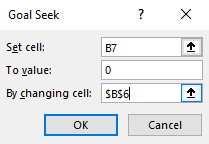
An Excel template solution for a Break-Even cash flow model. Suppose a firm can invest V0 = $1,000 present dollars in exchange for future dollars R1 = $200, R2 = $250, R3 = $350, and salvage value V3 = $950. Also assume that the defender exchanges dollars between time period at the rate of (1.08). The financial manager wants to know the salvage value that would allow the challenger to break even—to earn the defender’s IRR of 8 percent. To find the break-even salvage value solution, we introduce Excel’s goal seek solution described in the Excel appendix to this book.
We begin with the solution in Table 9.3. Then Goal Seek asks, if we require the value in cell B7, the investment’s NPV, to be set equal to zero, how much would we need to change the investment’s salvage value in cell B6 (the salvage value V3)?
| B7 | fx | =NPV(B1,B3:B4,(B5+B6))-B2 | |
|---|---|---|---|
| A | B | C | |
| 1 | r | 0.08 | |
| 2 | V0 | $1,000 | |
| 3 | R1 | $200 | |
| 4 | R2 | $250 | |
| 5 | R3 | $350 | |
| 6 | V3 | $950 | |
| 7 | NPV | $431.50 | =NPV(r,V0,R1,R2,R3+V3)-V0 |
| 8 | max bid | $1,431.50 | =V0 + NPV |
We report the goal seek solution in Table 9.5. We find that the salvage value could fall from $950 to $406.43 and still break-even, i.e., the challenger could earn the defender’s IRR of 8 percent and an NPV equal to zero.
| A | B | |
|---|---|---|
| 1 | r | 0.08 |
| 2 | V0 | $1,000 |
| 3 | R1 | $200 |
| 4 | R2 | $250 |
| 5 | R3 | $350 |
| 6 | V3 | $406.43 |
| 7 | NPV | $0.00 |
Annuity Equivalent (AE) Models
An annuity is a financial product sold by financial institutions. The essence of an annuity is this: an individual or firm pays into a fund that is invested and grows until some point when the investment is paid back to the investor as a constant stream of payments for a specified period. In this book we define a related concept, an annuity equivalent. An annuity equivalent is a constant stream of payments whose present value is equivalent to some other stream of payments that may not be constant. The annuity equivalent model finds an annuity associated with an investment. An annuity is like a time adjusted average. Suppose we wished to find the annuity equivalent associated with the generalized NPV model below:
(9.10) 
The value for R in equation (9.10) is the annuity equivalent (AE) cash flow. The discounted PV of the constant cash flow R yields an amount equal to NPV.
An Excel template solution for an AE model. Suppose a firm can invest V0 = $1,000 present dollars in exchange for future dollars R1 = $200, R2 = $250, R3 = $350, and salvage value V3 = $950. Also assume that the defender exchanges dollars between time period at the rate of 8 percent. Under this scenario, the firm estimates its NPV to equal $431.50. The financial manager wants to know what is the AE for an NPV of $431.50 over 4 years? The AE solution for this investment over 4 periods is $130.28, negative since it represents funds being withdrawn from the investment. We find AE using Excel’s PMT function.
| B9 | fx | =PMT(B1,B8,B7) | |
|---|---|---|---|
| A | B | C | |
| 1 | r | 0.08 | |
| 2 | V0 | $1,000 | |
| 3 | R1 | $200 | |
| 4 | R2 | $250 | |
| 5 | R3 | $350 | |
| 6 | V3 | $950 | |
| 7 | NPV | $431.50 | |
| 8 | n | 4 | |
| 9 | AE | ($130.28) | =PMT(r,n,NPV) |
The PMT solution informs us that an NPV of $431.50 could pay $130.28 for four years in the future before exhausting its value.
Capitalization Formulas
Long-lived assets, often non-depreciable, require a special PV model. Long-lived assets will be discussed in more detail in Chapter 14 on investment terms. But for now, consider the following. Suppose that we can considered the future cash flow of a long-lived asset to be represented by the annuity equivalent model described in equation (9.10). Now let n, the term of the investment, get very large. Then the present value of the present value of the AE can be written as:
(9.11) 
The capitalization formula, like all PV models that depends on future forecasts, is an approximation. In this case the approximation improves with increases in n. To illustrate suppose that we found the PV for n = 30, r = 8%, and AE = $130.28. The Excel solution is PV(.08,20,130.28) = $1,466.66. The capitalization approximation is $130.28/.08 = $1628.50. If n increases to 40, PV equals $1,553.54.
Optimal Life Models
Optimal life models ask what is the optimal life of this investment? We may want to ask if the NPV of the investment in equation (9.9) would be increased if the economic life of the investment were increased to the (n + 1) period or reduced to the (n – 1) period. The optimal life model in continuous time can be written as:
(9.12) 
Where R(t) equals the cash flow in the tth period and Sn is the salvage value in the nth period. The optimal solution has a specific meaning in the context of the optimal life model. It is that value of n that maximizes the NPV. Formally, the solution employs the calculus to optimize the NPV. In the discrete time model which is most often employed in practice, the optimal value is found through trial and error or through repeated calculations of alternative values for n.
A related optimal life model asks: what is the optimal value of n that maximizes NPV if there are replacements for the investment? In this case, NPV is the sum of NPVs from individual investments. Such a replacement model will be described in more detail in Chapter 14.
The Payback Model
While PV models are generally carefully deduced and the data required to solve them is explicit, sometimes decision makers just want a “ball-park” estimate of the desirability of a financial strategy. In such cases, decision makers are willing to sacrifice rigor and precision for approximations. When this is the case, the payback model is often employed. To obtain an approximation, it assumes the discount rate in PV models is zero. In other words, the payback model assumes that present and future dollars are valued the same—a very unrealistic assumption. Then the payback model calculates the number of periods required to earn the investment’s present value. The number of periods required to earn the investment’s value is the payback period, the criterion used to rank investments. All cash flow after the payback period is assumed to have no influence on the criterion. To illustrate, n is the payback period in the payback model that follows.
(9.13) 
And if periodic cash flows are constant we can express the payback period as:
(9.14) 
To illustrate, consider an initial outflow of $5,000 with $1,000 cash inflows per month. In this case, the payback period would be 5 months. If the cash inflows were paid annually, then the result would be 5 years. More generally, cash flows will not equal one another. If $10,000 is the initial outflow investment, and the cash inflows are $1,000 in year one, $6,000 in year two, $3,000 in year three, and $5,000 in year four, then the payback period would be three years, as the first three years are equal to the initial outflow.
Despite its popularity, the payback model is not recommended for several reasons. Mainly, ignoring the time value of money basically treats an inter temporal investment as though it were a static profit problem. Furthermore, it treats cash flow earned after the payback period as not important. In sum, in many respects, the pay-back method inadequately accounts for important details of the investment problem.
Present Value Models and Rates of Return
So far, the opportunity cost of capital has been introduced without specifying whose capital is being invested. Is it equity capital, debt capital, or a combination of debt and equity capital? Or does it matter? The short answer is that it does matter as we demonstrated in Chapter 8. If the focus is on the return on equity, then the discount rate represents the return on equity ROE in a one-period model and IRRE in a multi-period model. When focused on the rate of return on equity, interest costs on debt are subtracted from the cash flow included in the model. If the focus is on the return on assets ROA in a one-period model and IRRA in a multi-period problem, then the cost of the investment is subtracted at the beginning of the model and earnings reflect a return to the assets, and interest costs are irrelevant since the asset is treated as though it were purchased at the beginning of the investment.
The difference between the two approaches matter because most firms rely on a combination of debt and equity to fund assets. Reduced to its essence, the issue is whether the opportunity cost of capital reflects the rate of return on the firm’s assets or equity. Both approaches apply under different circumstances. For example, interest costs may be subsidized so that ROE estimates may be distorted compared to what they would be if the firm paid the market rate of interest. In this case, a return to asset approach may be appropriate. In other circumstances, the firm may indeed want to know their earnings and rate of return independent of contributions from debt capital. In this case, a return on equity approach may be appropriate. We now describe the two approaches in more detail using a one-period model to make the results transparent.
Internal rate of return on assets (ROA). In the return to asset model, we charge the entire investment at the beginning of the period and include its liquidation value as a return at the end of the period. This approach ignores the fact that investments may be financed and paid for over the life of the investment and charging for the investment at the beginning of the project doesn’t accurately reflect its cash flow. However, in the ROA approach, we ignore financing because our interest is in the productive capacity of the long-term asset, independent of the terms under which it can be financed. The advantage of the ROA approach is that the analysis considers the rate of return on the entire investment made at the beginning of the period. The NPV for the ROA approach for a single period can be expressed as:
(9.15) 
Note that in equation (9.15), if NPV = 0, as it would in an IRR model, then (1 + ROA)V0 is equal to R1 + S1. If we replace V0 with E0 + D, we can write R1 + S1 = (1 + ROA)(E0 + D). This fact will be helpful as we connect ROA and ROE measures.
We illustrate how to find ROA in a simple one-period example. Suppose the firm’s defender is a $1,000, non-depreciable investment that will earn $100 for one period and then will be liquidated at its acquisition price. We find the ROA associated with $1,000 of assets invested in the defender by setting its NPV equal to zero in equation (9.15) and solve for ROA.
(9.16) 
Internal rate of return on equity (ROE). In the ROE approach, the analysis depends on how the asset is financed. In this approach, the cost of interest and debt payments are subtracted explicitly. Moreover, the initial investment is equal to the amount of equity invested since the debt is paid directly to whoever supplies the investment. However, the debt D plus average interest costs charged at interest rate i (iD) are subtracted at the end of the period. The NPV for the one-period ROE model is expressed as
(9.17) 
Now reconsider the same example, except that the $500, or half of the defender, is financed at 9%. The other half of the investment, $500, is financed by the firm’s equity. We continue to assume that, after one period, the investment is liquidated for its acquisition value, the loan of $500 is repaid, and the firm recovers its investment of $500. The firm also earns in one period, $100, the same as before. But now it pays a rental fee for the use of the loan’s funds of 9% times $500, or $45. By setting the NPV model of the defender in equation (9.17) equal to zero, we can find its ROE associated with the firm’s equity (IRRE) in the project equal to.
(9.18) 
We find the defender’s ROE to equal 11%. In this case, the firm gained access to the use of an asset because of financing. The gains from a lender providing the firm access to $500 of debt capital to acquire a $1,000 investment using only $500 of its own money increased its earnings on its equity from 10% to 11%. Meanwhile the investment as a whole continued to earn only 10%. The value of the financing increased the rate of return on equity by 1%.
For a variety of reasons, financial managers may prefer to represent the defender’s rate of return using ROA. However, this same manager must be careful to make sure that the cash flow associated with the challengers are consistent and measure cash flow earned by assets. On the other hand, if the defender’s rate of return is represented by its ROE, then debt and interest costs should be accounted for explicitly.
In practice, most PV modelers appear to prefer the ROA approach, even though both approaches are valid and provide unique information. Nevertheless, the dominance of the ROA approach has resulted in the identification of ROAs as simply the IRR of the investment, a practice we will also adopt in the remainder of this book.
Summary and Conclusions
This chapter reviewed several different kinds of PV models. They differ because they are designed to answer different kinds of questions. Some PV models, NPV and IRR, help us rank alternative investments. Others like AE models can be used to find the optimal time for replacing an investment—or what our periodic loan payments will be. And still other PV models like the maximum bid (minimum sell) models help us know the maximum (minimum) we can offer to purchase (sell) an investment and still earn the defender’s IRR. Finally, still other PV models such as capitalization formulas and payback models offer at most a rule of thumb for evaluating and making investment decisions.
Questions
- PV models can be identified by the questions they are designed to answer. Please complete the table below by identifying the unknown variable and the question the solution to the unknown variables is designed to answer:
| Question you want to answer | Unknown Variable | Appropriate PV Model to Answer your Question |
| What is the rate of return I can expect from my equity invested in a lawn care business? | ||
| What will be my loan payment for a $10,000 loan to be repaid in 10 annual installments at an interest rate of 6%? | ||
| How much will the value of my assets change if I disinvest $50,000 from a defender and reinvest the funds in a challenger, assuming my defender is earning an IRR of 9%? | ||
| What is the most I can pay for a challenging investment and break-even or earn my defender’s IRR? | ||
| I own an aging orchard. I need to know the optimal time to replace my orchard with new tree varieties. | ||
| I am considering the purchase of beef feeder operation. I want to know the value of the operation realizing that I will earn returns on many beef-feeder cohorts. | ||
| If the discount rate is zero, how many periods will be required to recover my original investment. |
- Compare the implied reinvestment rates for NPV and IRR models.
- IRR models measure an investment’s internal rate of return. NPV models measure the difference in present earnings between the defender and the challenger. Both NPV and IRR models can be used to rank investments. Would you expect them to ranking investments consistently? Defend your answer.
- To find the present value of a stream of future income for a long-lived asset, I capitalize the constant or first period’s cash flow. What are the key assumptions employed that permit us to use the capitalization formula?
- Suppose you found the maximum bid price for a purchase you are considering. How would you use this information in your negotiations with the seller?
- Suppose that you found that an investment’s AE reached its maximum at year 10 while its NPV reached its maximum at 15 years. How would you use these results to determine the optimal life of the investment?
- When finding the ROE, we explicitly accounted for the debt used to finance the investment. However, when finding the ROA measure, we did not account for the debt used to finance the investment. Explain the difference between the two approaches. Which one would you recommend?
- Provide numerical PV models in which you find an investment’s IRR and NPVs using IRRA and IRRE.
- Most of the time, we don’t identify discount rates in PV models as being either a ROE or a ROA. Instead we seem to prefer to identify the defender’s ROA with the letter “r”. Why do we tend to prefer ROA to ROE measures? Can you describe a case when it would be important to evaluate the projects using the defender’s ROE instead of its ROA?
- Assume you were considering one investment that could be financed from two different financial institutions. Thus, the only difference between the projects were their cash flow associated with their use of debt capital. How would you proceed to rank the two investments?
