Forecasting and Present Value Models

Lindon Robison

11 Forecasting and Present Value Models

Lindon Robison

Learning goals. At the end of this chapter, you should be able to: (1) distinguish between deterministic and statistical forecasts; (2) recognize the difference between endogenous and exogenous variable forecasts; (3) recognize the difference between dependent and independent variables in statistical forecasts; (4) recognize the value of quantitative forecasts; (5) understand how to apply economic theory to guide forecasts, and (6) be able to complete present value (PV) models by forecasting endogenous and exogenous variables.

Learning objectives. To achieve your learning goals, you should complete the following objectives:

Understand the difference between forecasts and predictions.
Be able to recognize different kinds of deterministic and statistical forecasts.
Recognize the difference between exogenous and endogenous variables and forecasts.
Distinguish between independent and dependent variables in regression equations.
Learn the difference between quantitative forecasts and qualitative predictions.
Understand why present value (PV) models require cash receipts and cash expense forecasts.
Learn how to find forecast confidence intervals.
Utilize information about time and use costs to forecast cash costs of goods sold (COGS) and overhead expenses (OEs).
Understand how to use correlations among variables to make forecasts.
Practice forecasting techniques for simple investment problems.

Introduction

^[1]

Forecasts and predictions. This chapter is about forecasting. Forecasts use observations and perceptions about the past to predict the future. The origin of the word forecast comes from the word “fore” which means before plus the word “casten” which means to scheme, plan, or prepare. Thus, when we forecast, we predict something before it happens so that we can plan or prepare for it.

Related to forecasts are predictions. A prediction is also a statement about what someone believes will happen in the future. We sometimes distinguish between predictions and forecasts based on how we arrived at our estimate of the future. A prediction is a guess, less scientific, and more subjective than a forecast. In this view, predictions are more eclectic in the information they collect and use to describe the future–including past observations, informed opinions, conditional relationships, signs, impressions, and other foreshadowings of the future.

Everyday forecasts. We all make forecasts. We depend on them. Indeed, nearly every choice we make is preceded by a forecast. We are so dependent on our almost “every moment” forecasts that we may give them little notice. For example, we may give little thought to our forecast that if we turn on the water faucet, then water will pour out. Still our forecast precedes and motivates our act of turning on the faucet.

The relative importance of forecasts. What makes some forecasts more important than others are when they lead to significant resource commitments and are costly if not impossible to reverse. Buying a house, a new car, or choosing one’s companion may fall into the category of important forecasts. When making important forecasts, we may need to make several related forecasts. In the case of buying a car, we may want to forecast its frequency of repairs, its fuel efficiency, its riding comfort, and rather it impresses our partner. To improve our car-related forecasts, we may visit with friends who have made similar purchases. We may read professional car buying guides that evaluate the performance and cost of alternative cars of interest. We may even rent the car of interest to experience the car upfront and personal. But at the end of the day, we forecast our car purchase experience and make our choice—and live with the results.

Forecast accuracy. The accuracy of our forecasts varies depending on the quality of information and analysis behind them and the time distance to the future forecast. Consider the following. Because we have a long history of turning on the water faucet and experiencing the flow of water, we may be nearly certain of the relationship between turning on the faucet and experiencing the flow of water. In this case, the accuracy of our forecast is high. On the other hand, we may have heard that an eatery serves a tasty Rueben sandwich and based on the “expert” opinions of our friends, we may forecast that if we eat the Rueben at the eatery, we will be pleased with the experience. In this case the accuracy of our forecast is moderate. (Who is to say that our friends have the same tastes in sandwiches that we do?) Some forecasts are embedded in advertisements—that by consuming certain products, you will become popular and rich and your skin blemishes will disappear. These forecasts should be questioned unless supported by double-blind studies—because they are not motivated to report accurate results.

Forecasting, a two-step procedure. Forecasting is a two-step procedure. In the first step, we collect and analyze data to discover variables are related to each other over time. Suppose we observe an exogenous variable at time t, x_t, and find that it is significantly correlated with the same variable in the previous periods. Then we could write: x_t = f(x_t-1,x_t-2,⋯) + ε_t where ε_t is an error term that represents what is not explained by the exogenous variable in the current and adjacent time periods.

Suppose that in the first step, we forecast a value for x_t that we designate as x̂_t since it is an estimate because we don’t know what the actual value is. Then to estimate two periods in the future we solve using coefficient we found in step one to find: x̂_t+1 = f(x̂_t,x_t-1,⋯). In the case that x̂_t+1 – x̂_t = c then our forecast k periods in the future is: x̂_t+k = x̂_t + kc.

What follows. In what follows, we distinguish between different forecast equations based on the nearly certain information that provides the basis for our forecasts. While all forecast equations provide estimates of the future, some of them are derived deterministically and some statistically. In the case of statistically estimated forecast equations, it will be important to distinguish between dependent and independent variables. When describing the kinds of variables forecast, we will use the earlier language of Chapters 5 and 7, to distinguish between exogenous and endogenous variables. The purpose of this chapter is, at the end of the day, to find the forecasted endogenous and exogenous variables required to complete PV models. Questions at the end of the chapter can be used to practice and gain some forecasting experience.

Forecast Equations

Exogenous and endogenous variables. Exogenous variables are defined outside of a system. Endogenous variables are defined within the system. When we constructed coordinated financial statements (CFS) and PV templates, we distinguished between variables whose values were determined within the CFS and PV template, endogenous variables, and those variables whose values were determined outside of the CFS and PV template, exogenous variables. Within both the CFS system and PV templates, endogenous and exogenous variables are related to each other using deterministic equations.

Dependent and independent variables. When conducting experiments, it is common to use the language of dependent and independent variables. Independent variables are controlled by the experimenter and varied to determine their influence on dependent variables related to independent variables by statistical models. However, sometimes the relationship between dependent and independent variables is not determined experimentally but inferred and observed. This is the sense that we use dependent and independent variables in forecast equation.

Independent variables and what do we know for sure? We require independent variables to forecast dependent variables. Our independent variables are those used as exogenous variables in the CFS and PV templates used to determine endogenous variables. So, what independent variables do we know for sure? There are only two things that we know for sure that can be used as independent variables in our forecast equation: the time distance to a future date and the values of variables already realized, including lagged values of the dependent variable. If we were to include a contemporaneous variable to our independent variables in our forecast equation, we would need to forecast it as well as the dependent variable. This sometimes occurs when large forecast models forecast several dependent variables using multiple equations. In our discussion, we limit our forecasts to single equations. Finally, our confidence in the correlation between our dependent variables and time and lagged values increases with the quality and quantity of information used to infer the correlations.

Still, human behavior can often be predictable—we often act the same way in similar circumstances, and we develop habits that seem ingrained. We often use these tendencies to aid us in our forecasts. One important category of events that we use to guide our forecasts are commitments and covenants to perform in a predictable way in the future. For example, most have borrowed and agreed to repay on loans following specified terms. These performance commitments can be treated as nearly time dependent exogenous variables.

Forecasting endogenous variables. While forecasts mostly focus on exogenous variables when used within CFS and PV templates, we may find it useful to forecast endogenous variables. Forecasting endogenous variables is usually not necessary because they are determined by relationships established within the CFS and PV template. However, we recognize that our exogenous variables are estimated with error so that endogenous variable forecasts derived from the exogenous variable forecasts also contain errors. As a result, we may find it useful to over-identify some endogenous variables and a check on accuracy of our exogenous variables.

So, what have we learned? We learned that system variables may be either exogenous variables determined outside of the system or endogenous variables determined within the system by exogenous variables. Exogenous variables used to determine endogenous variables are dependent variables forecast by statistical or other models using independent variables that have been observed or that are highly correlated with the passage of time. In sum, we are mostly interested in forecasting exogenous variables (for our purposes) to use in CFS or PV templates. While we could technically, forecast endogenous variables, and sometimes we do, they are not our primary concern because they are determined within the CFS or PV templates.

In what follows, we will organize our forecast equation around what we know for sure. As a result, some forecast equations depend only on the passage of time. Others depend on the lagged values of a dependent variables. And still others depend on the lagged values of independent variables. Finally, we may create hybrid forecast equations that combine time and lagged values of dependent and independent variables. Forecasts that combine contemporaneous independent variables require accompanying equations that forecast their values—forecast equations in which they are the dependent variables.

Forecast Equations and What we Know

Trend lines. Consider forecasting exogenous variables that are highly correlated with or are dependent on the passage of time. Time may enter the forecast equation in several different forms, but to forecast future periods only requires time as the independent variable. An example may be an equation that forecasts the condition of a building’s roof k periods in the future. The condition of the roof and its remaining life might both be expressed as a function of the roof’s age. Consider such an expression:

A roof’s remaining useful life equals its useful life when constructed – it age.

Forecast equations that depend mostly on the passage of time are often referred to as trend lines. In this case, the endogenous variable y depends only on a constant and the independent variable t. This forecast equation can be expressed as:

(11.1) $\begin{equation*} y_t = \theta_0 + \theta_1 t + \epsilon_t \end{equation*}$

The trend line forecast k periods in the can simply be written as:

(11.2) $\begin{equation*} \hat{y}_{t+k} = \theta_0 + \theta_1 (t + k)\end{equation*}$

In equation (11.2), the hat over the endogenous variable signifies that we have an estimate, not an actual value.

Lagged dependent variable. Suppose that Lon wants to forecast the demand for his services next season. His forecast might begin with the demand for his services he experienced during the previous period. One reason to emphasize the demand for Lon’s services in the previous period is because so many conditions that existed last year will exist this year. To reflect the connection between this year’s forecast and what happened last year, we specify:

Services in period t = services provided in period (t – 1) + an error term

To complicate our forecasts, we recognize that the change in demand for Lon’s services in period t will depend on the number of new lawn care providers (Lon’s competition) plus change in the number of potential customers measured by the number of new households in Lon’s service area with a yard. Call these changes in the demand less changes increases in services provided by others equal to change in services ∆s_t and write the result as:

Services in period t =services provided in period t – 1 + ∆s_t + error.

Distributed lags of independent variables. Closely related to forecasts that depend on the passage of time and lagged values of depend variables are lagged values of independent variable on which the dependent variable depends. This forecast equation is relevant when the dependent variable depends on the outcome of other independent variables. Some variables such as costs of goods sold (COGS), depend on production activities in the previous period. So, if we intend to forecast COGS, we may want to relate them to some function of production activities in the previous period.

COGS this period = some function of production activity levels in the previous period.

A popular forecast equation that combines both the lagged dependent variable and independent variables is the infinite geometric distributed lag (IGL) forecast equation. We derive it next.

Suppose we want to forecast a dependent variable at the end of period t, y_t, whose value we assume depends on the infinite lagged values of an independent variable z, z_t-1,z_t-2,z_t-3,⋯ weighted by the geometric factor |ρ|<1. In this case we can write our forecast equation as:

(11.3) $\begin{equation*} y_t = \alpha + \beta (z_t + \rho z_{t-1} + \rho^2 z_{t-2} + \cdots) + \epsilon_t \end{equation*}$

where α, β, and ρ are estimated coefficients. Without simplifying (11.3), it would be nearly impossible to estimate. However, using the geometric series sum technique, we can simplify (11.3) to an equation that we can estimate. To simplify, we lag (11.3) to obtain

(11.4) $\begin{equation*} y_{t-1} = \alpha + \beta (z_{t-1} + \rho z_{t-2} + \rho^2 z_{t-3} + \cdots) + \epsilon_{t-1} \end{equation*}$

Then if we multiply (11.4) with ρ and subtract the result from (11.3), we obtain the geometric sum of the lagged values of z and an equation that we can estimate:

(11.5) $\begin{equation*} y_t - \rho y_{t-1} = \alpha - \rho \alpha + \beta z_t + \epsilon_t - \rho \epsilon_{t-1} \end{equation*}$

Solving for the current value of the endogenous variable and letting the error term equal v_t = ε_t – ρε_t-1 we can write:

(11.6a) $\begin{equation*} y_t = \alpha (1 - \rho) + \rho y_{t-1} + \beta z_t + v_t\end{equation*}$

And

(11.6b) $\begin{equation*} y_t = \gamma_0 + \rho y_{t-1} + \beta z_t + v_t \end{equation*}$

and where α = γ₀ / (1–ρ). In addition, the proper estimation of equation (11.6b) and other linear regression models requires that the error term, in this case ν_t, is distributed normally with a zero mean and a variance of σ², a condition we express as N(0,σ²).

The geometric lag. The geometric lag structure that produced equation (11.6b) is specific. More general lag structures can be estimated. Indeed, another geometric lag structure is (z_t-1 + ρz_t-2 + ρ²z_t-3 + ⋯) that produces the model in equation (11.7) that doesn’t require a forecasted value of z to estimate y and can be expressed as:

(11.7) $\begin{equation*} y_t = \gama_0 + \gamma_1 y_{t-1} + \gamma^2 z_{t-1} + v_t \end{equation*}$

Forecasting exogenous variables using time and lagged values as independent variables. We have already described forecasting as a two-step procedure. The first step requires that we find the relationship between dependent variables and lagged dependent variables, time and/or lagged value of other relevant variables calculated using past observations. The second step requires that we project the forecast dependent or exogenous variable into the future. If the independent variable is time, then to find a forecast requires only that we update our time variables. On the other hand, if our independent variable includes lagged values, then we must forecast using a stepwise procedure. In the first step we find our next period forecast. In the second step our forecast becomes the independent variable in our two-period future forecast—and so on to obtain future in the future forecasts. To illustrate, suppose that in the first-step we estimated that:

(11.8) $\begin{equation*} \hat{x}_t = a + bx_{t-1} \end{equation*}$

Then in the second step, our first period forecast becomes the independent variable is our two- period forecast allowing us to write:

(11.9) $\begin{equation*} \hat{x}_{t+1} = \alpha + \beta \hat{x}_t \end{equation*}$

Repeating the substitution process, we obtain a k period in future forecast equal to:

(11.10) $\begin{equation*} \hat{x}_{t+k} = \alpha + \beta \hat{x}_{t+k-1} \end{equation*}$

It should be noted that in equation (11.8), the forecast was only one period away from something we knew for sure, the lagged value of dependent variable. In equation (11.9) we were two periods away and in equation (11.10) we were k periods away from something we knew for sure. Therefore, we might conclude that the further away from lagged values we know for sure, the less confidence we should have in the accuracy of our forecast.

Deterministic versus linear regression forecasting equations. There are two ways to process data that describes the relationships between dependent and independent variables. The first method assumes that our relationship that describes the connection between dependent and independent variables is measured without error and the forecast is deterministic. The second method assumes that the relationship between dependent and independent variables approximates the true relationship which we don’t know. So, in this second case, the best we can do is to estimate statistically the relationship between the dependent and independent variable(s) and recognize that the actual forecast is a sophisticated guess. We will refer to these methods here that explicitly recognize we are not completely accurate in our estimation of the dependent and independent variable relationship as a statistical regression model.

Several factors determine whether we should forecast using a deterministic or a regression model. These factors may include our confidence in our data, the importance of our forecasts, and difficulty and cost of gathering and processing the data. In what follows, we describe and give examples of both deterministic and linear regression models.

Deterministic Forecasts

A naïve forecast. Assume that the relationship between a dependent variable y is a linear function of itself lagged equal to:

(11.11) $\begin{equation*} y_t = a + by_{t-1} \end{equation*}$

If we are unable or unwilling to estimate coefficient a and b in equation (11.11), we may assume their values to equal: a = 0 and b = 1. This assumption implies that y_t = y_t-1. We call this a naïve forecast.

Even though the deterministic naïve forecast is our simplest forecast, it has its place. Suppose our question is: what would be the consequences on the investment’s value if everything continued as it is right now? The answer to that question may indeed be a naïve (constant value) forecast. We demonstrate a naïve forecast using Lon’s services provided during the previous four years. These are represented in Table 11.1. Our forecast description includes the actual value x_t, the forecast x̂_t , and the error of the forecast ϵ_t.

**Table 11.1. Deterministic naïve forecasts of Lon’s service calls**
Time period	Actual value x_t	Forecast vales x̂_t	Forecast error: ϵ_t = x_t – x̂_t
0	525	n.a.
1	755	525	230
2	890	755	135
3	990	890	100
Forecast	n.a.	990	n.a.

One test of the accuracy of one’s forecast is the pattern of the forecast error. We expect it to be randomly distributed about zero—in this case the sum of errors should be close to zero. In this case the sum of errors equal 365. In this case, our forecast model fails the test, and so we try a different forecast model.

Moving average forecasts. A step up in forecast sophistication that does not rely on statistical methods is the moving average. Suppose that we are interested in predicting the amount of services Lon could provide if the business continued another year. If we truly believed there was no trend in the data and the variation was due to random events, we might reduce the random effects on the forecast by averaging the previous four period (990 + 890 + 725 + 525)/4 = 782.5 or possible the last three (990 + 890 + 755)/3 = 878.3 or perhaps the most recent two observations (990 + 890)/2 = 940. However, because there is a positive trend, a weighted average forecast is even less accurate than the naïve forecast of 990 over the sample period, and we have no way of knowing its accuracy of the forecast beyond the sample period.

Geometric forecasts. PV models by their nature are geometrically designed created by compounding discount rates of the form ab, ab¹, ab²,⋯, abⁿ where a and b are constants and superscripts represent the geometric factor. As a result, we may assume that our forecasts should also follow some form of a geometric series.

To make geometric forecasts, we begin by observing previous values of exogenous variable values reported in current and past Coordinated Financial Statements (CFS). To illustrate, suppose that over the past 10 years, corn yields g₁, g₂, ⋯, g₁₀ have increased by 13%. Then letting g̅ equal the average percentage increase in corn yields we find the average yield in equation (11.12) equal to:

(11.12) $\begin{equation*} (1 + g_1)(1 + g_2) \cdots (1 + g_n) = (1 + \bar{g})^n \end{equation*}$

Where g_t is the actual growth rate in the exogenous variable for periods t = 1,⋯,n and the average geometric growth rate is g̅. To illustrate suppose we had growth rates of corn yields for 10 year that we represent as:

(11.13) $\begin{equation*} (1 + g_1)(1 + g_2) \cdots (1 + g_10) = (1.13) = (1 + \bar{g})^n \end{equation*}$

Then solving deterministically for the average geometric mean over the past ten years of yields, we find:

(11.14) $\begin{equation*} (1 + \bar{g}) = (1.13)^{0.1} = 1.0123 \end{equation*}$

Or an average, for the past 10 years, yields in period t that we represent with the variable y_t increased by 1.23%. Assuming the past trends in yield continue and if the yield last year were 140 bushels per acre, in 5 years we would expect yields to have increased to:

(11.15) $\begin{equation*} y_5 = 140(1.0123)^5 = 148.82 \end{equation*}$

In other words, corn yields in period 5, assuming the average yield trend for the past ten years continues will equal 148.82 bushels per acre. In the case of Lon’s services, over four years services have increased by 990/525 = 200% or 1.89^0.3 = 1.26 of that services have increased on average by 26 percent per year so that next year’s forecast for Lon’s business is (990)(1.26) = 1,221.

Linear Regression Forecasts

What is a linear regression forecast? The second forecasting method is the statistical procedure referred to as multiple linear regression or in the case of a single explanatory variable, linear regression. Regression analysis finds a coefficient for a line (plane) through points representing values of a dependent variable such that the squared differences between the line and the values of the regression line are minimized. Hence, the regression method is sometimes referred to as least squares regression analysis.

Regression models can also be used to measure the percentage of the total variation around the mean of the data explained by regression equation using what is referred to as an R² that is between zero and 100 percent. Obviously, as we add more independent variables to our regression equation, we can increase the value of R². However, as we add independent variables to our regression equation, the significant of each individual independent variable will likely decrease, a significance measured by t-tests. Eventually, we can add enough independent variables that our relationships is deterministic. When conducting regression analysis, we assume that independent variables are measured without error and not influenced by each other. Dependent variables are related to the independent variables and we expect them to be forecast with some error.

Finally, the ability to estimate regression equations are often complicated by missing variables, non-normal distributions of υt, autocorrelations between the error terms and correlations between the error terms and the exogenous variables and other properties keep econometricians occupied. These complications and others encountered when estimating regression equations, we ignore in this chapter in order to emphasize the fundamental concepts of forecasting.

A Lagged Regression Model and Forecast. Suppose we return to equation (11.11) and instead of assuming coefficient values of a = 0 and b = 1 we estimate coefficients a and b in regression equation (11.16).

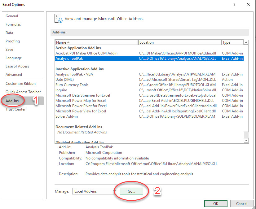
(11.16) $\begin{equation*} y_t = a + by_{t-1} + \epsilon_t \textrm{ where } \epsilon_t ~ N(0,\sigma^2) \end{equation*}$

Fortunately, Excel has a statistical function that can estimate a and b so that the sum of ε_t² is is minimized and the sum of ε_t’s is zero. To access regression analysis for estimating regression coefficient a and b in Excel we select Data and regression from the drop-down menu. If the Analysis tab does not appear, it may be necessary to access it from your options. Instructions to enable this option are in the appendix at the end of this chapter.

Microsoft Excel Data Menu Ribbon showing Data Analysis Button — **Figure 11.1. Data Ribbon for Excel Spreadsheet**

After selecting the Data tab, select regression from the drop-down menu.

Pop-up menu after selecting Data Analysis button on the Data Ribbon showing Regression selected.. — **Figure 11.2. Data Analysis Pop-up Menu**

After selecting regression from the drop-down menu, we are asked for regression analysis data. The lagged independent values for x_t-1 (A2:A4) are entered in the Input X Range. The current or dependent values x_t (B2:B4) are then entered as the Input Y Range:

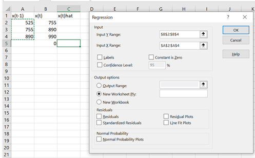
We include a request that the regression equation find the constant value a. Clicking OK returns the regression estimates for our forecast equation equal to:


	A	B	C	D	E	F	G
1	Summary Output
2
3	Regression Statistics
4	Multiple R	0.997992
5	R Square	0.995989
6	Adjusted R	0.991978
7	Standard	10.56297
8	Observation	3
9
10	ANOVA
11		df	SS	MS	F	Significance F
12	Regression	1	27705.09	27705.09	248.3061	0.040346
13	Residual	1	111.5763	111.5763
14	Total	2	27816.67
15
16		Coefficients	Standard Error	t Stat	P-value	Lower 95%	Upper 95%
17	Intercept	417.0247	29.90354	13.94567	0.045572	37.06427	796.9852
18	X Variable (t)	0.637754	0.040472	15.75773	0.040346	0.123503	1.152005

Interpreting all the output described above is beyond the scope of this discussion and the proper topic for a beginning econometrics class. However, note that R² accounts for most of the variation in the data and the t-tests for the coefficients a and b are greater than 1.9 which is often reported as the minimum required for the independent variables to be retained.

Having found the forecast equation, we use the results to obtain our forecasts. To do so, we focus on the estimates of coefficient a reported in cell B17 equal to 417.02 and coefficient b reported in cell B18 equal to .638.

(11.18) $\begin{equation*} \hat{x}_t = a + bx_{t-1} = 417.2 + .638x_{t-1} \end{equation*}$

Next we create our table of lagged values, estimated values, errors, and a forecast value.

**Table 11.3. Naïve forecasts of Lon’s service calls**
Time period	Actual value x_t	Estimated and Forecast vales x̂_t	Forecast error: ϵ_t = x_t – x̂_t
0	525	n.a.
1	755	752	3
2	890	899	-9
3	990	985	5
Forecast	n.a.	1049	n.a.

Notice that we obtain our forecast for x_t-1 by substituting our last observed value of 990 into our forecast equation:

(11.19) $\begin{equation*} \hat{x}_t = a + bx_{t-1} = 417.2 + .638(990) = 1049. \end{equation*}$

Notice that accounting for a trend line significantly improved our estimated values over the sample range compared to previous forecast equations. Furthermore, the error term appears more nearly random and sums to a number close to zero: 3 – 9 + 5 = 1. However, before we become too impressed with our estimates compared to our actual values, we must acknowledge that we have only three estimated values to estimate the two unknown parameters “a” and “b”. In other words, we almost have a perfectly identified systems so there is really no estimating challenge at all leaving us with a lack of confidence that our three-year trend will really continue.

Nonlinear trend lines. It is common for most new business to make impressive gains early on and then see gains level off. Indeed, it appears that for many processes, growth appears to follow a concave down pattern as might be described in the graph below.

Trend line with steep increases that levels off. — **Figure 11.4. Quadratic Trend Line.**

Such a function can be represented with a more complicated mathematical representation like the one below:

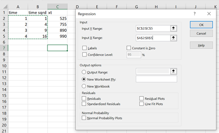
(11.20) $\begin{equation*} y_t =\beta_0 + \beta_1 t + \beta_2 t^2 \end{equation*}$

Notice for the exogenous variable time and time squared, we entered the data matrix. Next we click OK to obtain the result:


	A	B	C	D	E	F	G
1	Summary Output
2
3	Regression Statistics
4	Multiple R	0.999259
5	R Square	0.998518
6	Adjusted R	0.995554
7	Standard	13.41641
8	Observation	4
9
10	ANOVA
11		df	SS	MS	F	Significance F
12	Regression	2	121270	60635	336.8611	0.038498
13	Residual	1	180	180
14	Total	3	121450
15
16		Coefficients	Standard Error	t Stat	P-value	Lower 95%	Upper 95%
17	Intercept	245	37.3497	6.559625	0.09631	-229.573	719.5729
18	X Variable (t)	315.5	34.07345	9.259409	0.068488	-117.444	748.4442
19	X Variable (t²)	-32.5	6.708204	-4.84481	0.129583	-117.736	5273581

We are particularly interested in the coefficient for our estimated equation (11.21). We write the results as:

(11.21) $\begin{equation*} \hat{x}_t = a + bt +ct^2 = 245 + 315.5t = 32.5t^2. \end{equation*}$

We create our table of lagged values, estimated values, errors, and a forecast value.

**Table 11.5. Forecasts of Lon’s service calls based on a quadratic function of time.**
Time period	Actual value x_t	Estimated and Forecast vales x̂_t	Forecast error: ϵ_t = x_t – x̂_t
1	525	528	-3
2	755	746	9
3	890	899	-9
4	990	987	3
Forecast	n.a.	1010	n.a.

Note that the forecast based on a quadratic function of time is 1010 compared to 1049 based on a linear function of time. Since both equations report significant R² and t-values—we must choose between them based on economic logic—which model best fits the reality on the ground?

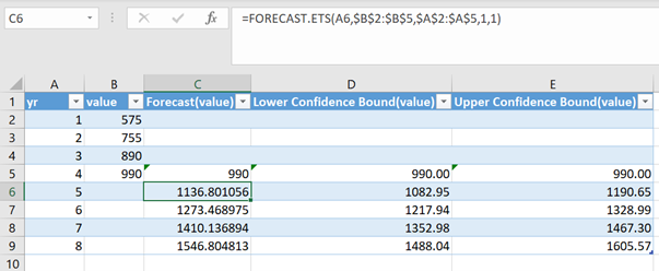
Confidence intervals. Assume the new potential owner is unsure about the reliability of the forecasts and asks what are the high and low forecast values? Using the forecast.confidence function, we can find statistical bounds around the projected trend line using the standard deviation of values around the trend link. Then we add and subtract the standard deviation multiplied by a constant such that given data and assuming the trend continues, we can be 95% sure that the “true” projection is included in the bounded confidence interval. Below we include the forecast values for Lon’s services during the next four year. Then we graph the original values, their forecasted values and the confidence intervals.

Excel table showing values for years 1 through 4 and then forecast values for years 5 through 8. — Table 11.6. Forecast values for the demand for Lon’s Green & White Services for the next four years, and 95% confidence intervals around the forecasts.

Forecasts and Shocks

Exogenous variable forecasts and shocks. Now suppose that in time t + k we forecast the value of our dependent variable but something we call a shock, s_t+k, occurs that hasn’t occurred in the past. Because the shock hasn’t occurred in the past, we don’t account for it in our forecast. Or suppose something that has occurred in the past that helped us forecast y_t+k doesn’t occur? This is another kind of a shock.

To illustrate the first kind of shock, consider Christmas tree sales. Based on our past experiences, we forecast a significant rise in Christmas tree sales in December. But suppose this year, the world experiences a pandemic and tree-harvesters are quarantined and unable to supply the usual number of Christmas trees. Then we may find that our Christmas tree sales forecast to be widely inaccurate.

Shocks may have two kinds of consequences. And the kinds of forecasting consequences shocks may produce depend on what we are forecasting. If we are forecasting a quantitative value—e.g. Christmas tree sales, our forecast may be inaccurate such as we observe a reduction is sales of 50% below our forecast. Or, if we are forecasting an event with only two possible outcomes, e.g. win or lose, then our forecast is either right or wrong, correct or incorrect, true or false. Such would be the case if we forecast the winner of the Super Bowl and the wrong team wins. In this case, are forecast was not merely inaccurate, it was wrong.

Getting real. Before proceeding, we need to get real. Relationships between endogenous and exogenous variables are hardly ever stable or easily identified. Remember shocks? To illustrate, assume that we intended to forecast future corn prices. We begin by identifying the connection between past corn prices and other past exogenous variables. But then, we might find the relationship that we thought we had estimated was not stable and susceptible to forces not included in our model including shocks. Corn prices fell by two and one-half times in the 1970s leading to a fall in related prices and the financial crisis of the 1980s. Land values fell as much as 50 percent during the same time period. Later, in the 2006–2013 period corn prices nearly doubled over the previous twenty-year period only to fall again in 2013 with input prices substantially higher than in the previous period. In real terms, current profitability was lower than it was in the post 1980’s period. Historically, it has taken grain and oilseed markets six to twelve years to find their “new normal” following large, sustained shocks. History again provides a guide to the future, but the internal confidence around these future projections should be wide.

Recognizing the difficulty of what we’re about, in what follows we employ equation (11.1) beginning with its most simple form and then consider increasing complicated forecast equations. Our goal is to find first the relationship between endogenous and exogenous variables to forecast their future values.

So, what have we learned? We have learned that forecasts depend on their values being highly correlated with the passage of time where we determined the correlation between t and independent variables by past observations. However, things in the future may not be just like they were in the past. Things that happened in the past that we assumed will happen in the future, don’t. Or things that didn’t happen in the past, do happen in the future. Both unplanned events we call shocks. So, in time period t+k, instead of observing y_t+k, we observe y_t+k + s_t+k. What is the influence of a shock on our forecast depends on if we are forecasting discrete outcomes (win versus lose) or continuous values (the level of Christmas tree sales).

Forecasting Exogenous Variables and the Accuracy of Endogenous Variables

Earlier we distinguished between dependent and independent variables in forecast equations and exogenous and endogenous variables in CFS and PV templates. When the exogenous variables are known in CFS and PV templates, endogenous variables are found using deterministic equations. We now ask, what about exogenous and endogenous variables in CFS and PV models when exogenous variables are forecast with error. Now we are less confident that the deterministic relationships from which we find endogenous variables as some deterministic function of exogenous variables can still be relied on?

We propose that we establish some over-identified checks on the values of our endogenous variables as means of validating our exogenous variable forecasts. In practice this proposal means that we use economic reasoning and other established relationships between endogenous and exogenous variables to obtain independent estimates of our exogenous variables besides the deterministic one obtains from CFS and PV templates. In other words, once we have obtained forecasts for our exogenous variable(s) x̂_t, we are prepared to use these forecasts to find the future values of our endogenous variables ŷ_t.

These conditional forecasts of our endogenous variables take the form: if x(t) then y(t). To illustrate, we may forecast umbrella sales to increase if it rains—if it rains then umbrella sales will increase. We may not be able to predict the weather, but we can predict how consumer purchases will likely respond to the occurrence of rain. In the statement, if x̂(t) then ŷ̂(t), x̂(t) is the exogenous variable forecast and ŷ̂(t) is the endogenous variable forecast.

Another illustration of a conditional forecast, the forecast of an endogenous variable, may be the firm’s profit forecasts. An agricultural firm’s profit forecast may depend on several factors including weather, crop yields, trade policies, inventory levels, input costs, revenue and expense margins, and national economic variables such as stock market indices, consumer price indices, consumers’ disposable incomes, the interest rate, and the level of consumer confidence to name a few.

Once we have obtained our exogenous variable forecasts from deterministic or regression equations, we now intend to use these to forecast future values of endogenous variables. The connection between exogenous and exogenous variables may be deterministic as was their calculations in CFS and PV templates. In other cases, they simply may be related to each other statistically even though economic logic may lead to the equation that forecasts endogenous variables from the base of exogenous variables.

Sometime correlations with exogenous variables can be useful even if the exogenous variable is not one with which we are directly interested. This is because several exogenous variables may be influenced in similar ways by time. Prices are a case in point. Some prices seem to move together through time and this correlation may be particularly helpful in our endogenous variable forecasts. In these cases, the relationship between exogenous and endogenous variables are not deterministic and must be estimated.

Price forecasts. In our original study of Lon’s service, we predicted prices to be constant over the four years of Lon’s operations. This forecast is naïve. Instead, suppose that we believed that Lon’s prices for services would follow national price trends. One national price trend is the consumer price index (CPI). The CPI measures changes in the price level of a weighted average market basket of representative consumer goods and services purchased by households. There are, of course, several different CPI indexes. To calculate the CPI, we designate a base year for prices and assign it an index of 100. Then the updated value of the index is found by dividing the index of prices is the updated period by the index of prices in the base year:

(11.22) $\begin{equation*} \dfrac{CPI_t}{CPI_{base}} = \dfrac{\textrm{Average Prices}_t}{\textrm{Average Prices}_{base}} \approx \dfrac{\textrm{Lon's prices}_t}{\textrm{Average Lon's Prices}_{base}} \end{equation*}$

Suppose that we wish to know the average percentage increase from the base year to year t. If the current CPI were 123% and the base year were 10 years earlier, we could find the average geometric increase in prices to be those we found earlier:

(11.23) $\begin{equation*} (1 + \bar{g}) = (1.23)^{(1/10)} = 1.02\end{equation*}$

In other words, prices (including the price of lawn care services) have increased by 2% per year. If we applied this estimated average of prices to yard care services, we can forecast Lon’s future price for yard care services:

**Table 11.7. Forecast values for the price of Lon’s Green & White Services Assuming a 2.1% increase**
Year	Forecast Service Prices	Service times forecast price = sales	COGS = .45 x sales
Base	$40
1	$40.84	$40.84 x 525 = $21,441	$965
2	$41.69	$41.69 x 755 = $31,476	$14,164
3	$42.67	$42.67 x 890 = $37,976	$17,089
4	$43.46	$43.46 x 990 = $43,025	$19,361

Percentage forecasts and margins. One of the main ways we can forecasts endogenous variables outside of the CFS and PV template is to observe the relationships between them and exogenous variables in the past—and the more observations, the better. One observation that is important using past data is the margin between revenue and costs. We can be confident that this difference is bounded, otherwise, competitors would flock to join our industry and begin replicating our operations. If the difference is negative for some time, we will become insolvent and forced to leave the industry. Sometimes, if we can discover the connection between margins and time—we may forecast margin as a function of time. For example, suppose we are interested in the price of hard red winter wheat but can only observe past prices of corn and soybeans. Using linear regression, a statistical technique that allows us to relate an endogenous variable to one or more exogenous variable—we can use the future estimates of corn and soybean prices to predict hard red winter prices.

Sales data. In column three of Table 11.1 and beginning in year one, we estimate cash sales or cash cost reductions. We can employ several assumptions about future cash flow associated with sales or reduced costs. The first one is that there is no change from data entered in year one. This assumption is consistent with capitalization formula that assume zero change in future cash flow. It may also be relevant if the model assumes that data are in real numbers so that numbers do not change with inflation. Furthermore, we may assume the future is represented by the present and these relationships between variables in the present should be preserved.

Economic logic and margins. Economic logic and margins may guide our endogenous variable forecasts. Recall that common size income statements provide us percentage relationships between endogenous and exogenous variables. Consider the common size income statement for HQN. Such a statement could, of course, be acquired for other industries more nearly like the industry in which we are focused.

**Table 11.8. (Table 7.9) HQN’s Accrued Common-Size Income Statements**
Year	2017	2018	Industry Average
Total Revenue	100.00%	100.00%	100.00%
Cost of Goods Sold (COGS)	67.37%	70.00%	71.40%
Operating Expenses	29.82%	27.50%	22.50%
Depreciation	1.24%	0.88%	1.75%
EARNING BEFORE INTEREST AND TAXES (EBIT)	1.58%	1.62%	4.35%
Interest	1.22%	1.20%	0.55%
EARNINGS BEFORE TAXES (EBT)	0.36%	0.42%	3.80%
Taxes	0.17%	0.17%	1.52%
NET INCOME AFTER TAXES (NIAT)	0.19%	0.25%	2.28%

Economic logic suggests that some relationships between exogenous and endogenous variables may continue in the future. For example, taxes are likely to be function of the difference between revenue and sales. Another class of relationships likely to persist over time are margins, 100% minus the percent of costs as a function of revenue. Economic logic tells us that margins can’t be zero or negative or the firm wouldn’t survive. Nor can they be excessively high without inviting competitors and innovators to join the industry. Of course, changing competitive advantages and innovations may temporarily affect margins, in the short run and will likely encourage changes in the industry as firms expand to take advantage of the innovations. And as we increase in sophistication, we might. worry about local, national, and international politics that may influence tariffs and the challenges of competing in a global economy—ultimately affecting our margins.

COGS and Revenue. The foundation for our forecasts is the economic relationship between the variables in our industry. Once we have price and/or yield forecasts, we can add other forecasts by treating them as dependent variables. Two variables of economic necessity must be highly correlated are costs and revenue. For example, we may expect to find that COGS has a predictable relationship to sales since the more we produce and sale the more expenses we are likely to occur. Therefore, once we have sales forecasts, we can forecast COGS using established relationships observed from past data.

One other relationship is the difference between revenue and costs. We can be confident that this difference is bounded. Otherwise, if the difference were strongly positive, competitors would flock to our industry and begin replicating our operations. If the difference is negative for a significant period of time, we will become insolvent and leave the industry. Taxes will be some function of the difference between revenue and sales. Changes in comparatives advantages and preferences may also be included in the description of how the variables are related. Future preferences will influence demand for what we produce.

Changes in comparative advantage—who can produce least expensively and where—will also influence revenue and expenses. Favorable increases in comparative advantage will reduce our costs and put us in a position to expand our operation. And as we increase in sophistication, we might worry about local, national, and international politics that may influence tariffs and the challenges of competing in a global economy.

Consider COGS in Table 11.1. In this example, we estimated COGS to be on average 45% of sales. Sales have been forecast to increase by 3 percent from base sales we observed in the CFS that described the firm. As a result, COGS will also increase by 3% maintaining a constant relationship of 45% between sales and COGS.

Still another method for estimating future cash revenue and expense cash flow is to employ someone else’s guesses about the future. This is difficult because our investment and earning potential is often unique to our own firm. Still there are guesses about the future that are related to our own investment’s future. And there are sophisticated forecasting firms and experts who make predictions about the future relevant to our own investment. For example, a dairy firm might be interested in forecasted milk prices or the expected cost of feed. Firms related to home sales would find future interest rate forecasts to be relevant since the demand for homes can be expected to be related to the cost of home financing. Indeed, most investments can be tied to some future forecast that is relevant.

COGS and OE. Associated with the business include what economists refer to as fixed and variable costs. We treat COGS as variable costs that follow the investment’s cash revenue. In addition, we impose on the relationship between CR and COGS the restriction that long-term, Sales>COGS. OE are costs difficult to assign to any one production activity and vary over time. In our simplified analysis, we did not assume any OE. This is an unreasonable assumption since such fixed costs such as insurance, rental of office and storage space, and licenses all produce fixed costs. In the previous four years, fixed costs were $350, $390, $450, $515. In addition, in the most recent two years, Lon was required to rent addition space that cost $100 in each period. We use the OE observations and estimate the following equation using our observed data.

(11.24) $\begin{equation*} OE = \alpha_0 + \alpha_1 \textrm{time} + \alpha_2 \textrm{ additional storage} \end{equation*}$

The way our forecasts work in practice is that we find some historical basis for the equation and from those relationships estimate our coefficients.

Now we illustrate the various forecasting methods using the data in our example template. To begin, suppose that we are confident in the cash flow data appearing in year two since year one may be a transition year. Dividing cash COGS by cash sales we find:

(11.25) $\begin{equation*} 0 < \gamma < \dfrac{COGS}{\textrm{Cash Sales}} = \dfrac{\$106,913}{\$137,068} = 78\% \end{equation*}$

As a result, in the future, we will assume that COGS equal 78% of whatever we estimate sales to equal. Whatever we estimate sales to equal, we will assume that COGS equal

Other forecasts. Sometimes, failing to find forecasts of direct interest to the calculation of our investment’s NPV, AE, and IRR—we can often find forecasts highly correlated with our forecasts of interest. For example, suppose we are interested in the price of hard red winter wheat but can only observe past prices of corn and soybeans. Finding past relationships between the price of hard red winter wheat and corn and soybean prices, we can use forecasts of corn and soybean prices to forecast future prices of hard red winter wheat.

Real versus nominal data values. In our PV templates, we project CR, cash COGS and cash OE. We can employ several assumptions about future cash flow associated with these values. The first one is that there is no change from data entered in year one. This assumption is consistent with capitalization formula that assume zero change in future cash flow. It may also be relevant if the model assumes that data are in real numbers so that numbers do not change with inflation. Furthermore, we may assume that the future is represented by the present and these relationships between variables in the present should be preserved.

Testing for robustness. That we populate our PV templates with estimates suggests that our templates will not be completely accurate. They will be consistent because the templates relate variables to each other consistently, but they are not likely to be completely accurate. We simply are not likely to estimate all of the future values of our variables correctly. As a result, we should calculate NPV, AE, and IRR under a variety of assumptions about future values so that we have some impression about the robustness of our estimates.

So, what have we learned? We have learned that forecasting recognizes two different kinds of statements. The first of these is of the form: if t then y_t. From this relationship between t and y_t, we make forecasts that include linear trend lines and other more complicated functions of time. Other kinds of forecast depend on lagged values of the dependent and independent variables.

We have been careful to distinguish between dependent and independent variables in forecast equations and exogenous and endogenous variables in CFS and PV templates. In the latter case, the relationship between exogenous and endogenous variables are deterministic that depend on accounting identities. The problem occurs that when we forecast exogenous variables, these are estimated with error that implies that our endogenous variables in CFS and PV templates are also estimated with error. Then it may be useful to find overidentified estimates of our endogenous variables to validate our exogenous variable forecasts—using the structure of our CFS and PV templates to check for accuracy. These require that we forecast our endogenous variables as well as our exogenous variables using economic and other logic to guide our estimation of endogenous variables. This type of estimation, like other forecasts will be of the form if x_t then y_t.

Qualitative Forecasts

Not everything we know can be reduced to a number. If all the lessons learned from the past could be translated into a quantitative forecast function, we could leave much of forecasting to computers (they already carry a significant forecasting role). But such is not the case. We all know much more that can be represented by a numerical forecast. When historical data is not available, we generally employ qualitative forecasting techniques that most often depend on the judgment of experts—that may be aided by quantitative forecasts.

Experts and all the rest of us observe, absorb, and process informative through our multiple sources and senses. So how do we do it? We may not be able to describe the process because our intuitive sense are complicated and profound. Book like “Thinking Fast and Slow” try to describe some aspects of our capacity to analyze and predict using information much more sophisticated that has been described in this chapter. This is not to disrespect the amazing information captured by digital coding, especially in the sciences, but when it comes to the “animal spirits” that operate in interpersonal interaction, it pays to leave room for qualitative judgments and forecasts.

So, we employ and appreciate professional forecasters to share their qualitative forecasts, sometimes augmented by quantitative forecasts. In may be the case that we will increasing translate qualitative forecasts into quantitative ones—and multitude are the examples of qualitative forecasts being improved using quantitative information.

Professional forecasts are usually experts in their specialty such a yields and prices of agricultural and forestry products as well as margins between revenue and cost. An example of expert forecast services are those offered by the Food and Agricultural Policy Research Institute (FAPRI) at the University of Missouri. FAPRI makes annual 10-year baseline projections for grain, oilseed, livestock markets, and a variety of other indicators. Even here, it is important to moderate forecasts using microeconomic principles and experience in making projections including a range of scenarios. Understanding intermediate and longer-term industry supply curves including regional and international dimensions is very important for most projects. Extension specialists, such as Dr. Jim Hilker, who have distinguished themselves with accurate forecasts can also be an invaluable resource.

One advantage of professional forecasts is that they account for so many influences that uncomplicated forecasters may ignore. The other advantage is that when we present our forecasts and responses to our forecasts are important—it is always helpful to have a reliable source for support.

PV Models and Forecasts

Forecasts and present value models. While this chapter is about forecasting, we are most interested in forecasting PV model exogenous variables. Solving PV models requires that we forecast the future value of cash flow generated by an investment. PV models include exogenous and endogenous variables.

PV models discount future cash flows to find their equivalent worth in the present—since it is in the present where we live and make decisions. To repeat for emphasis, we cannot solve PV models without forecasting future exogenous variable cash flow on which the present value of an investment depends. When we invest in the present, all we know for sure is the cost of the investment, the time distance to different futures, lagged values of endogenous and exogenous variables, and future commitments like loan terms. Every other piece of data requires us to solve the PV problem and exogenous variable forecasts.

To illustrate, the template below is identified as: PV Template: Green & White Services. It will be helpful in our forecasting discussions in this chapter to continue using Lon’s yard care investment example. We will embellish it somewhat to focus on certain aspects of forecasting while maintaining the main characteristics of the problem.

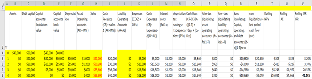
Screenshot of Excel Template. — **Table 11.9. PV Template: Green & White Services** Open PV Template in Microsoft Excel.

Data for Green & White Services. Looking to the future, Lon is considering the purchase of a lawn care/snow removal business. He will purchase the good will (customer base) of the previous owner of the business and equipment for $40,000. His expected service calls, service prices and variable cost per service are reported below:

**Table 11.10. Endogenous and exogenous variable forecasts for Green & White Services.**
	A	B	C	D	E	F	G	H	I	J	K	L	M	N
1	Year	Number of Services	Price/Service	Cost/Service	Sales	AR+INV	CR	Expenses	AP+AL	CE	Depreciation Rates	V0	Depreciation	Debt
2	1	525	40	18	21000	1000	20000	9450	100	9350	0.25	40000	10000	0
3	2	755	40	18	30200	1200	30000	13590	200	13490	0.375	40000	15000	0
4	3	890	40	18	35600	800	36000	16220	100	16120	0.25	40000	10000	0
5	4	990	40	18	39600	400	40000	17820	100	17820	0.125	40000	5000	0

Forecast number of services are described Table 11.10 column B. Prices and cost per service forecasts are described in columns C and D and when multiplied by projected services produce sales revenue in column E and expenses in column H. Note that these are accumulated sales and costs, not cash. The sum of accounts receivable (AR) and inventory (INV) at the end of the period are reported in column F while the sum of accounts payable (AP) and accrued liabilities (AL) are reported in column I. Cash receipts (CR) and cash expenses (CE) are found by adjusting sales and expenses for changes in asset and liability accounts and the results are recorded in columns G and J respectively. Allowable depreciation rates are recorded in column K and when multiplied by the capital asset purchase of $40,000 produce depreciation amounts recorded in M. Finally, debt outstanding is recorded in Column N.

Besides the annual data forecasts, we also record certain rate forecasts for Green & White Services. Some of these as well as some of the annual forecasts may be either exogenous or endogenous variables depending on how the endogenous defining equations are define. We include the current exogenous rates as:

**Table 11.11. IRRs, average tax rate, average interest rate, and growth rates is applicable for Green & White Services.**
	A	B
1	ROA	0.08
2	T	0.2
3	ROE(1-T)	0.064
4	Average Interest Rate	0.06
5	Debt Growth Rate	0
6	Liquid Growth Rate	0
7	Book Value Growth Rate	0
8	Account Balance Growth Rate	0
9	CR Growth Rate	0
10	COGS Growth Rate	0
11	OE Growth Rate	0
12	Beginning Cash	0
13	Liability op. Account Rate	0

We now ask, where can we find future values for template variables that will permit us to solve multi-period PV problems? The answer is that we forecast or estimate (guess) the value of exogenous variables in the template and based on these exogenous variable forecasts, we solve for the endogenous forecast variables.

Populating the PV template with exogenous and exogenous variables. Like Coordinated Financial Statements (CFS), we populate PV templates with exogenous and endogenous variables. The columns of data in Table 11.9 are organized into exogenous and endogenous variables. The exogenous variables are highlighted. Endogenous variables are not. The main distinction between exogenous and endogenous variables within the template is the following. The values of exogenous variables are determined outside of the template. The values of endogenous variables are determined within the main template. Excel makes it easy to distinguish between exogenous and endogenous variables. We can identify endogenous variables within the template because they require an operations such as +,-,*,^, or /. They may also require an operation embedded in an Excel function such as PV, PMT, NPER, RATE, IRR, or NPV.

Otherwise, they are exogenous. If the cell requires an operation, it will be signaled by an “=” sign that references other cells included in an operation. Exogenous variables may reference cells outside of the PV model with an equal sign when they contain values on which an operation will be performed. Alternatively, exogenous data cells in the template may include a number. The exception to this means for identifying endogenous variables is when they are calculated in separate pages and then copied into the main template.

We now describe in more detail the variables and data needed to populate our PV templates that enable us to find rolling NPV, AE, and IRR estimates for investments and invested equity. We begin with the only information we know for sure, future dates: 2019, 2020, 2021, etc. Therefore, we begin populating our PV templates with the one thing we know about the future: future dates recorded in column 1.

The investment acquisition amount. We record the investment acquisition amount in cell B4. Its value is determined outside of the template making it an exogenous variable. We treat the investment’s acquisition value as though it were a cash expenditure unless funded by debt, an amount recorded in cell C4. When we employ debt to acquire the investment, the focus is on the equity invested—equal to the investment amount less the debt used to acquire the investment.

If we purchased the investment(s) on credit, we enter the loan principal and interest payments in the years they are paid. We don’t enter the loan amount because money came from a lender and was received by the seller of the investment—Lon is only an intermediary in the exchange

The investment amount is also a well-documented number. Durable sellers post their offer prices. Markets establish and record the prices at which durables are exchanged. References for used durable prices like Kelly’s Blue Book for cars are generally available. Salvage values that occur sometime in the future are much harder to estimate. The IRS provides some economic life estimates and depreciation data equal to percent changes in the value of the original durable. Theses may help us establish book values and may provide some guide for determining the durables’ liquidation value.

Complicating our investment data are projects that incur investments costs over several time-periods. Indeed, one might consider repair and maintenance expenditures designed to improve the life and durable performance to represent additional investments. In other cases, the investment includes several durable that we replace at different intervals. For example, feeder calf operations routinely replace one cohort of calves with another but the feeding equipment and physical facilities we replace less often than the feed calves.

Liquidation values. To find rolling NPV, AE, and IRR estimates, we require not only an investment acquisition amount, but investment liquidation and market values over time. An investment’s acquisition value, V₀, is the amount of money exchanged to acquire the investment. An investment’s book value in period t, V_t^book, equals it acquisition value minus its accumulated depreciation. An investment’s liquidation value in period t, V_t^liquidation, is the amount of money a buyer is willing to exchange for the investment when it is sold. If an investment’s liquidation value is greater than its acquisition value, we refer to the difference as capital gains. If an investment’s liquidation value is less that its acquisition value but greater than its book value, we refer to the difference as depreciation recovery. Finally, if the liquidation value is less than its book value, we refer to the difference as capital losses. We describe capital gains, depreciation recovery, and capital losses in the following equations:

for V_t^liquidation > V₀ > V_t^book, capital gains = V_t^liquidation – V₀ > 0,

for V₀ > V_t^liquidation > V_t^book, depreciation recapture = V_t^liquidation – V_t^book > 0, and

for V₀ > V_t^book > V_t^liquidation, capital losses = V_t^book – V_t^liquidation > 0.

We determine accounting book values by applying tax regulations that specify depreciation amounts depending on the type and age of the investment. Since depreciation forecasts depend on the age and amount of the investment, we generally consider them endogenous variables. Furthermore, we recognize that liquidation values of investments are also generally determined by projecting market values and cost data and may be endogenously or exogenously variables. When we do not expect to liquidate the investments, but want to estimate their NPV, AE and IRR, we may equate market liquidation value with book values. That we populate our PV templates with forecasts, sophisticated guesses, suggests that our template is not completely accurate. As a result, we should calculate NPVs, AEs, and IRRs under a variety of guesses so that we have some impression about the robustness of our estimates.

Summary and Conclusions

We conclude this chapter with the observations that we are all forecasters—all the time. We are all today making decisions and plans that will influence our conditions in the future–and these require forecasts. As we review the nature of forecasts, we should be humbled by the process and two factors. The first one is that forecasts have been often wrong. As evidence, review the forecasts that predicted the great recession of 2008. And the second factor that should humble us is that the only thing we know for certain about the future is the time it will take us to get there.

We emphasize here that there exist many potential forecast equations. These should be evaluated based on their accuracy, their implementation difficulty, availability of data, and the importance of the forecast. Still, we need to accept that what should determine our confidence in the accuracy and correctness of our forecasts is finding exogenous variables highly correlated with the passage of time. Fortunately, there are several exogenous variables that are satisfy this requirement. Most natural phenomenon have some predictable life cycle patterns of growth, production, and decay. We all make commitments that commit us to some action in the future that we often complete. As a result, our own actions in the future can often be predicted. Still shocks often leave disturbs our confident in our forecasts.

Still, we must make decisions in the present that commit us to outcomes in the future—and there is no alternative. We will all continue to forecast and hope to become better in the effort. Hopefully, this chapter has provided some ideas on how we can all make better forecasts.

Questions

Describe the differences between forecasts and predictions.
How would you characterize the main business of forecasters?
List five forecasts and five predictions that you have made during the last week. Describe your confidence in the accuracy of your forecasts and predictions and what determined your confidence.
Forecasts can be accurate or inaccurate or wrong and right. Explain.
Evaluate the following forecast. A turkey woke up on Thanksgiving Day and forecast that it would be like every other day?
List two kinds of shocks. Provide an example from the nation news of the shocks.
Given the likelihood that not all of our forecasts will be accurate or correct, how can we plan these eventualities?
What is the difference between dependent and independent variables in forecast equations?
Explain the difference between exogenous and endogenous variables in the context of CFS and PV templates.
We may forecast exogenous and endogenous variables. Explain the difference in these forecasts and how they may be used.
Forecasting can be described as a two-step process.
The commodity price index is today 123 percent of its base 10 years ago.
1. Using a deterministic method, forecast the price index next year. If corn prices today are $3.18 forecast next year’s corn prices using the following methods:
2. Using a naïve forecast.
3. Using a geometric average forecast based on the commodity price index.
4. Assume that corn prices during the past four years were: $2.56, $3.90, $2.89. $3.25, and $2.89. Use a linear regression model to forecast corn prices next year and the year after next.
5. Using a regression equation with independent variables t and t^2 to forecast corn prices next year and the year after that.
6. Compare and comment of the R2 for the linear and quadratic function and the t statistics for coefficients of the independent variables in the equations.
Consider the PV template described in Table 11.1. Then resolve the template assuming that expenses (COGS +OEs) were an endogenous variable. Find the value of expenses using the exogenous variable sales data. Determine the relationship between COGS that vary with sales and OEs that mostly vary with the passage of time.
Assume the following endogenous and exogenous variables have been observed in the past. Forecast Y(7) using the data below. Determine the accuracy of your forecast and the confidence interval around your forecast.

Time Period	Y(t)	Y(t-1)	X(t-1)
1	45	35	44
2	52	45	39
3	67	52	33
4	68	67	34
5	80	68	26
6	78	80	21
7

Appendix

If the Data menu ribbon does not show the Data Analysis button at the far right, you can enable it in the Excel Options.

Excel Data menu ribbon without the Data Analysis option. — **Figure 11.A1. Excel Data Menu Ribbon without the Data Analysis option.**

Select File and then Options.

**Figure 11.A2. Excel File Menu Options Selection**

In the Excel Options popup window, first select the Add-ins menu, and then select the Go… button to Manage Excel Add-ins.

Excel Options with Add-ins menu and Manage Excel Add-ins highlighted. — **Figure 11.A3. Excel Options to Manage Add-ins.**

Finally, in the Add-ins popup window, check the Analysis ToolPak option and select OK.

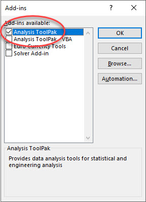
When you return to the Excel spreadsheet Data menu ribbon, the Data Analysis button is now available.

Excel Data Menu Ribbon with Data Analysis button enabled. — **Figure 11.A5. Data Ribbon with Data Analysis option enabled.**

Much of the material in this chapter was developed in an article under review by the Agricultural Finance Review titled: “Coordinated Financial Statements: What-is, What-if, and How-much Questions” by Lindon J. Robison and Peter J. Barry submitted January 2021. ↵

License

Icon for the Creative Commons Attribution-NonCommercial 4.0 International License

Financial Management for Small Businesses, 2nd OER Edition Copyright © 2021 by Lindon Robison is licensed under a Creative Commons Attribution-NonCommercial 4.0 International License, except where otherwise noted.