9 Climate Change

Weather vs. Climate

Although these words are often used interchangeably, they have very different meanings. View the following video to learn how they differ.

For closed captioning or to view the full transcript see the video on YouTube. Or click on the “YouTube” link in the video.

The Atmospheric Blanket and its Warming Effect

The gasses in the atmosphere act like a blanket, warming the earth and resulting in the natural greenhouse gas effect.

The Atmosphere

The Earth’s atmosphere is an extremely thin shell compared with the size of our planet. The primary gases in the atmosphere by volume are nitrogen (78.1%), oxygen (20.9%), and argon (0.9%). These figures don’t include water vapor, which varies significantly with location and altitude but averages about 0.4% of the atmosphere globally. Other naturally occurring gases include carbon dioxide (designated by chemists as CO₂), ozone, and methane, which all occur in trace amounts. Although CO₂, methane, and ozone occur naturally, human activities are increasing their concentrations. This blanket of atmosphere sustains life in many fundamental ways, as shown in the figure below.

The Natural Greenhouse Gas Effect

On the image below, click on the “question mark” hotspots to learn about solar radiation.

Not all of the emitted heat energy can escape to space. The greenhouse gases in the intervening atmosphere absorb (or trap) some of this heat energy. As a result, the heat energy leaving the planet is reduced by the intervening atmosphere. It is this trapping of heat energy that otherwise would have escaped to space through the atmosphere that is referred to as the greenhouse effect.

For closed captioning or to view the full transcript see the video on YouTube. Or click on the “YouTube” link in the video.

Learn More!

Read this interactive article by the Department of Environment, Great Lakes, and Energy to learn about Eunice Newton Foote: the woman who discovered greenhouse gases in the mid-1800’s.

Past Climate

Because scientists cannot go back in time to directly measure climatic variables, such as average temperature and precipitation, they must instead indirectly measure temperature. To do this, scientists rely on historical evidence of Earth’s past climate.

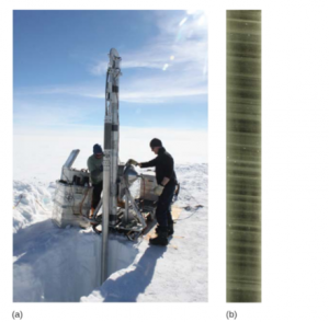
Antarctic ice cores are a key example of such evidence for climate change. These ice cores are samples of polar ice obtained by means of drills that reach thousands of meters into ice sheets or high mountain glaciers. Viewing the ice cores is like traveling backward through time; the deeper the sample, the earlier the time period. Trapped within the ice are air bubbles and other biological evidence that can reveal temperature and carbon dioxide data. Antarctic ice cores have been collected and analyzed to indirectly estimate the temperature of the Earth over the past 400,000 years.

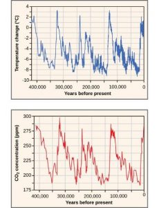
The 0°C on the graph below represents the long-term average. Temperatures that are greater than 0°C exceed Earth’s long-term average temperature. Conversely, temperatures that are less than 0°C are less than Earth’s average temperature. This figure shows that there have been periodic cycles of increasing and decreasing temperature.

Before the late 1800s, the Earth has been as much as 9°C cooler and about 3°C warmer. Note that the second graph below shows that the atmospheric concentration of carbon dioxide has also risen and fallen in periodic cycles. Also, note the relationship between carbon dioxide concentration and temperature. The graph shows that carbon dioxide levels in the atmosphere have historically cycled between 180 and 300 parts per million (ppm) by volume.

The figure above does not show the last 2,000 years with enough detail to compare the changes in Earth’s temperature during the last 400,000 years with the temperature change that has occurred in the more recent past. Two significant temperature anomalies, or irregularities, have occurred in the last 2,000 years. These are the Medieval Climate Anomaly (or the Medieval Warm Period) and the Little Ice Age. A third temperature anomaly aligns with the Industrial Era. The Medieval Climate Anomaly occurred between 900 and 1300 AD. During this time period, many climate scientists think that slightly warmer weather conditions prevailed in many parts of the world; the higher-than-average temperature changes varied between 0.10°C and 0.20°C above the norm. Although 0.10°C does not seem large enough to produce any noticeable change, it did free seas of ice. Because of this warming, the Vikings were able to colonize Greenland.

The Little Ice Age was a cold period that occurred between 1550 AD and 1850 AD. During this time, a slight cooling of a little less than 1°C was observed in North America, Europe, and possibly other areas of the Earth. This 1°C change in global temperature is a seemingly small deviation in temperature (as was observed during the Medieval Climate Anomaly); however, it also resulted in noticeable climatic changes. Historical accounts reveal a time of exceptionally harsh winters with much snow and frost.

The Industrial Revolution, which began around 1750, was characterized by changes in much of human society. Advances in agriculture increased the food supply, which improved the standard of living for people in Europe and the United States. New technologies were invented that provided jobs and cheaper goods. These new technologies were powered using fossil fuels; especially coal. The Industrial Revolution starting in the early nineteenth century ushered in the beginning of the Industrial Era. When fossil fuel is burned, carbon dioxide is released. With the beginning of the Industrial Era, atmospheric carbon dioxide began to rise.

Climate Models

Predictions about climate are created using climate models.

How We Use Models

Models help us to work through complicated problems and understand complex systems. They also allow us to test theories and solutions. From models as simple as toy cars and kitchens to complex representations such as flight simulators and virtual globes, we use models throughout our lives to explore and understand how things work.

Climate Models, and How They Work

Climate models are based on well-documented physical processes to simulate the transfer of energy and materials through the climate system. Climate models, also known as general circulation models or GCMs, use mathematical equations to characterize how energy and matter interact in different parts of the ocean, atmosphere, and land. Building and running a climate model is a complex process of identifying and quantifying Earth system processes, representing them with mathematical equations, setting variables to represent initial conditions and subsequent changes in climate forcing, and repeatedly solving the equations using powerful supercomputers.

Climate Model Resolution

Climate models separate Earth’s surface into a three-dimensional grid of cells. The results of processes modeled in each cell are passed to neighboring cells to model the exchange of matter and energy over time. Grid cell size defines the resolution of the model: the smaller the size of the grid cells, the higher the level of detail in the model. More detailed models have more grid cells, so they need more computing power.

See an animation showing different grid sizes »

Explore information about supercomputer systems used to run global climate models »

Climate models also include the element of time, called a time step. Time steps can be in minutes, hours, days, or years. Like grid cell size, the smaller the time step, the more detailed the results will be. However, this higher temporal resolution requires additional computing power.

How are Climate Models Tested?

Once a climate model is set up, it can be tested via a process known as “hind-casting.” This process runs the model from the present time back into the past. The model results are then compared with observed climate and weather conditions to see how well they match. This testing allows scientists to check the accuracy of the models and, if needed, revise their equations.  Science teams around the world test and compare their model outputs to observations and results from other models.

Using Scenarios to Predict Future Climate

Once a climate model can perform well in hind-casting tests, its results for simulating future climate are also assumed to be valid. To project climate into the future, the climate forcing is set to change according to a possible future scenario. Scenarios are possible stories about how quickly the human population will grow, how land will be used, how economies will evolve, and the atmospheric conditions (and therefore, climate forcing) that would result in each storyline.

In 2000, the Intergovernmental Panel on Climate Change (IPCC) issued its Special Report on Emissions Scenarios (SRES), describing four scenario families to describe a range of possible future conditions. Referred to by letter-number combinations such as A1, A2, B1, and B2, each scenario was based on a complex relationship between the socioeconomic forces driving greenhouse gas and aerosol emissions and the levels to which those emissions would climb during the 21st century. The SRES scenarios have been in use for more than a decade, so many climate model results describe their inputs using the letter-number combinations.

In 2013, climate scientists agreed upon a new set of scenarios that focused on the level of greenhouse gases in the atmosphere in 2100. Collectively, these scenarios are known as Representative Concentration Pathways or RCPs. Each RCP indicates the amount of climate forcing, expressed in Watts per square meter, that would result from greenhouse gases in the atmosphere in 2100. The rate and trajectory of the forcing is the pathway. Like their predecessors, these values are used in setting up climate models.

Learn more about RCPs »

Results of Current Climate Models

Around the world, different teams of scientists have built and run models to project future climate conditions under various scenarios for the next century. The model results project that global temperature will continue to increase, but show that human decisions and behavior we choose today will determine how dramatically climate will change in the future.

How are Climate Models Different From Weather Prediction Models?

Unlike weather forecasts, which describe a detailed picture of the expected daily sequence of conditions starting from the present, climate models are probabilistic, indicating areas with higher chances to be warmer or cooler and wetter or drier than usual. Climate models are based on global patterns in the ocean and atmosphere, and records of the types of weather that occurred under similar patterns in the past.

View maps showing short-term climate forecasts »

IPCC (Intergovernmental Panel on Climate Change)

The Intergovernmental Panel on Climate Change (IPCC) is the most prominent international scientific body for assessing climate change. It was formed in 1988 by the World Meteorological Organization (WMO) and the United Nations Environment Programme (UNEP). There are currently 195 member-countries in the IPCC, and membership is open to all countries in the WMO and UN. The IPCC is responsible for reviewing and evaluating scientific, technical, and socioeconomic information related to climate change. While the IPCC neither conducts research nor monitors any climate change data directly, it provides policymakers with the most comprehensive picture of the scientific consensus.

IPCC’s Climate Assessment Report

Working Group 1: Physical Science Basis

Working Group 1 investigates past, present, and future climate.

• Figure SPM.1 Temperature: a) The observed annual and decadal average temperature from 1850 to 2012, compared to the average for 1961 to 1990. Negative values indicate average temperatures were below the 1961-1990 average and positive values indicate above that average. b) World map of the observed change in surface temperature from 1901 to 2012.
• Figure SPM.2 Precipitation: World maps illustrating the change in precipitation from 1901 to 2010 and 1951 to 2010.
• Figure SPM.3 Cryosphere (snow and ice): For the 20th century, a) the amount of spring snow cover in the Northern Hemisphere, b) the extent of Arctic summer sea ice, c) change in global average upper ocean heat content relative to 1970, and d) change in global average sea level relative to 1900-1905.
• Figure SPM.4 Carbon Dioxide: a) Atmospheric concentration of carbon dioxide and b) surface ocean carbon dioxide and pH (the lower the number, the more acidic).
• Figure SPM.5 Drivers of Climate Change: Anthropogenic and natural climate change drivers and their impacts in 2011 compared to 1750.
• Figure SPM.6 Natural and Anthropogenic Impact: Global and regional graphs illustrating the impact of natural forcings and combined natural and anthropogenic forcings.
• Figure SPM.7 Predicted Temperature: Predicted temperature changes relative to 1986-2005 using four models (each model represents a different scenario (from cutting all carbon emissions today to not changing carbon emissions at all).
• Figure SPM.8 Predicted Climate: World maps showing predicted changes in climate for 2081-2100 relative to 1986-2005 for two different scenarios for a) temperature, b) precipitation, c) Northern Hemisphere September sea ice extent, and d) ocean surface pH (lower values mean more acidic).
• Figure SMP.9 Predicted Sea Level Rise: Graph depicting predicted sea-level rise using four models (each model represents a different scenario (from cutting all carbon emissions today to not changing carbon emissions at all).
• Figure SMP.10 Carbon Dioxide and Temperature: Global surface temperature correlated with temperature change relative to 1861-1880.
• See the WG1 SMP figures in context with full captions.

Working Group 2: Impacts, Adaptation, and Vulnerability

Working Group 2 investigates how changes in climate impact the environment and society.

• Figure SPM.2 Widespread Impacts: A world map illustrating how different regions are impacted by climate change.
• Figure SPM.5 Species Migration: The maximum speeds that species can move across landscapes compared to how quickly temperatures are expected to change.
• Figure SPM.6 Fisheries: Predicted climate change impact on a) catch potential and b) change in pH and which taxa are most impacted.
• Figure SPM.7 Crop Yield: Predicted climate change impact on future crop yields.
• Figure SPM.8 Solution Model: A model illustrating risks and mitigations.
• See the WG2 SMP figures in context with full captions.

Working Group 3: Mitigation of Climate Change

Working Group 3 investigates how we may reduce future climate change and the impact of its effects.

• Figure SPM.1 Greenhouse Gases: Total annual greenhouse gases by type: fossil fuel and industrial processes, forestry and other land use (FOLU), nitrous oxide (N₂O), and fluorinated gases covered under the Kyoto Protocol (F-gases).
• Figure SPM.2 Economic Sectors: Direct and indirect carbon dioxide emissions by economic sector.
• Figure SPM.4 Baseline and Mitigation Scenarios: Global greenhouse gas emissions for four scenarios: baseline (not changing our emissions path), two scenarios with varying emission levels, and one scenario for if we stopped carbon emissions.
• Figure SPM.9 Investment: Changes in annual investment flows projected for 2010-2029 based on keeping carbon dioxide emissions in a range of about 430 to 530 parts per million.
• See the WG3 SMP figures in context with full captions.

Attributions

This chapter is a modified derivative of the following articles:

“Climate and The Effects of Global Climate Change” by OpenStax College, Biology 2e, CC BY 4.0. Download the original article for free at https://openstax.org/books/biology-2e/pages/1-introduction

“Climate Models” by Climate.gov, NOAA, Public domain.

“Climate Change” by Ramanathan, V., Bending the Curve: Climate Change Solutions Digital Textbook, 2019, CC-BY-NC-SA.