
5 Gravity and falling objects
Esperanza Zenon; James Boffenmyer; Mostafa Elaasar; and Shirley Vides
Learning Objectives
-
Describe the effects of gravity on objects in motion.
-
Describe the motion of objects that are in free fall.
-
Calculate the position and velocity of objects in free fall.
-
Explain Earth’s gravitational force on objects.
-
Describe how the Moon’s gravity affects Earth.
-
Understand the concept of weightlessness in orbit.
-
Examine the Cavendish experiment and the measurement of [latex]G[/latex].
-
State and interpret Kepler’s three laws of planetary motion.
-
Derive Kepler’s third law for circular orbits using Newton’s laws.
-
Understand the historical context and limitations of the Ptolemaic model of the universe.
Falling objects form an interesting class of motion problems. For example, we can estimate the depth of a vertical mine shaft by dropping a rock into it and listening for the rock to hit the bottom. By applying the kinematics developed so far to falling objects, we can examine some interesting situations and learn much about gravity in the process.
Gravity
The most remarkable and unexpected fact about falling objects is that, if air resistance and friction are negligible, all objects fall toward the center of Earth with the same constant acceleration, regardless of their mass. This experimentally confirmed result often surprises those accustomed to thinking that heavier objects fall faster.
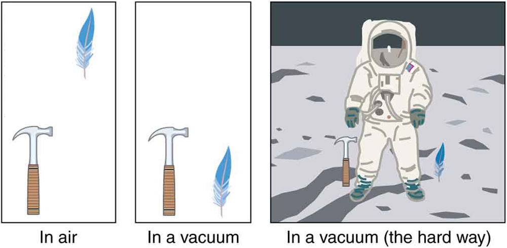
In everyday life, air resistance causes lighter objects to fall slower than heavier ones. For example, a tennis ball will typically hit the ground after a hard baseball dropped from the same height. In idealized situations—those we analyze first—air resistance and friction are ignored, and such an object is said to be in free fall.
The force of gravity causes all free-falling objects to accelerate toward the center of Earth. This acceleration is constant at a given location and is called the acceleration due to gravity, denoted by [latex]g[/latex]:
[latex]g = 9.80, \text{m/s}^2[/latex]
Although the precise value of [latex]g[/latex] varies slightly with location (from about [latex]9.78, \text{m/s}^2[/latex] to [latex]9.83, \text{m/s}^2[/latex]), we will use [latex]9.80, \text{m/s}^2[/latex] as the standard value throughout this text unless otherwise specified.
The direction of [latex]g[/latex] is downward—toward Earth’s center—and it defines what we consider the vertical direction. When working with kinematic equations, the sign of [latex]g[/latex] depends on your choice of coordinate system:
-
If upward is positive: [latex]a = -g = -9.80, \text{m/s}^2[/latex]
-
If downward is positive: [latex]a = g = 9.80, \text{m/s}^2[/latex]
One-Dimensional Motion Involving Gravity
To understand free-fall motion, we start with the simplest scenario: motion that is straight up or down, with no air resistance or friction. This means the velocity is purely vertical.
If an object is dropped (i.e., released without being thrown), then its initial velocity is:
[latex]v_0 = 0[/latex]
Once the object is released, it is in free fall. The acceleration is constant and equal to the magnitude of [latex]g[/latex].
We use [latex]y[/latex] to represent vertical displacement (rather than [latex]x[/latex], which we reserve for horizontal motion). The kinematic equations for vertical free-fall motion under constant acceleration become:
Kinematic Equations for Free-Fall Motion
-
Velocity after time [latex]t[/latex]:
[latex]v = v_0 - gt[/latex]
-
Displacement after time [latex]t[/latex]:
[latex]y = y_0 + v_0 t - \frac{1}{2} g t^2[/latex]
-
Velocity-displacement relationship:
[latex]v^2 = v_0^2 - 2g(y - y_0)[/latex]
Example 5.1: Calculating Position and Velocity of a Falling Object: A Rock Thrown Upward
A person standing on the edge of a high cliff throws a rock straight up with an initial velocity of [latex]13.0\ \text{m/s}[/latex]. The rock misses the edge of the cliff as it falls back to Earth. Calculate the position and velocity of the rock [latex]1.00\ \text{s}[/latex], [latex]2.00\ \text{s}[/latex], and [latex]3.00\ \text{s}[/latex] after it is thrown, neglecting the effects of air resistance.
Strategy
Draw a sketch.
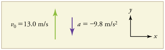
We are asked to determine the position [latex]y[/latex] at various times. It is reasonable to take the initial position [latex]{y}_{0}[/latex] to be zero. This problem involves one-dimensional motion in the vertical direction. We use plus and minus signs to indicate direction, with up being positive and down negative. Since up is positive, and the rock is thrown upward, the initial velocity must be positive too. The acceleration due to gravity is downward, so [latex]a[/latex] is negative. It is crucial that the initial velocity and the acceleration due to gravity have opposite signs. Opposite signs indicate that the acceleration due to gravity opposes the initial motion and will slow and eventually reverse it.
Since we are asked for values of position and velocity at three times, we will refer to these as [latex]{y}_{1}[/latex] and [latex]{v}_{1}[/latex]; [latex]{y}_{2}[/latex] and [latex]{v}_{2}[/latex]; and [latex]{y}_{3}[/latex] and [latex]{v}_{3}[/latex].
Solution for Position [latex]{y}_{1}[/latex]
- Identify the knowns. We know that [latex]{y}_{0}=0[/latex]; [latex]{v}_{0}=\text{13}\text{.}\text{0 m/s}[/latex]; [latex]a=-g=-9\text{.}{\text{80 m/s}}^{2}[/latex]; and [latex]t=1\text{.}\text{00 s}[/latex].
- Identify the best equation to use. We will use [latex]y={y}_{0}+{v}_{0}t+\frac{1}{2}{\text{at}}^{2}[/latex] because it includes only one unknown, [latex]y[/latex] (or [latex]{y}_{1}[/latex], here), which is the value we want to find.
- Plug in the known values and solve for [latex]{y}_{1}[/latex].
[latex]y{}_{1}\text{}=0+\left(\text{13}\text{.}\text{0 m/s}\right)\left(1\text{.}\text{00 s}\right)+\frac{1}{2}\left(-9\text{.}\text{80}\phantom{\rule{0.25em}{0ex}}{\text{m/s}}^{2}\right){\left(1\text{.}\text{00 s}\right)}^{2}=8\text{.}\text{10}\phantom{\rule{0.25em}{0ex}}\text{m}[/latex]
Discussion
The rock is 8.10 m above its starting point at [latex]t=1\text{.}\text{00}[/latex] s, since [latex]{y}_{1}>{y}_{0}[/latex]. It could be moving up or down; the only way to tell is to calculate [latex]{v}_{1}[/latex] and find out if it is positive or negative.
Solution for Velocity [latex]{v}_{1}[/latex]
- Identify the knowns. We know that [latex]{y}_{0}=0[/latex]; [latex]{v}_{0}=\text{13}\text{.}\text{0 m/s}[/latex]; [latex]a=-g=-9\text{.}{\text{80 m/s}}^{2}[/latex]; and [latex]t=1\text{.}\text{00 s}[/latex]. We also know from the solution above that [latex]{y}_{1}=8\text{.}\text{10 m}[/latex].
- Identify the best equation to use. The most straightforward is [latex]v={v}_{0}-\text{gt}[/latex] (from [latex]v={v}_{0}+\text{at}[/latex], where [latex]a=\text{gravitational acceleration}=-g[/latex]).
- Plug in the knowns and solve.
[latex]{v}_{1}={v}_{0}-\text{gt}=\text{13}\text{.}\text{0 m/s}-\left(9\text{.}{\text{80 m/s}}^{2}\right)\left(1\text{.}\text{00 s}\right)=3\text{.}\text{20 m/s}[/latex]
Discussion
The positive value for [latex]{v}_{1}[/latex] means that the rock is still heading upward at [latex]t=1\text{.}\text{00}\phantom{\rule{0.25em}{0ex}}\text{s}[/latex]. However, it has slowed from its original 13.0 m/s, as expected.
Solution for Remaining Times
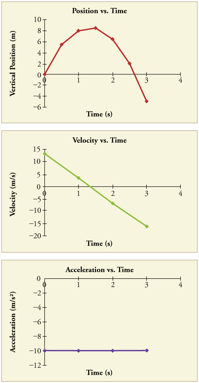
The procedures for calculating the position and velocity at [latex]t=2\text{.}\text{00}\phantom{\rule{0.25em}{0ex}}\text{s}[/latex] and [latex]3\text{.}\text{00 s}[/latex] are the same as those above. The results are summarized in Table 5.1 and illustrated in Figure 5.3.
Graphing the data helps us understand it more clearly.
Discussion
The interpretation of these results is important. At 1.00 s the rock is above its starting point and heading upward, since [latex]{y}_{1}[/latex] and [latex]{v}_{1}[/latex] are both positive. At 2.00 s, the rock is still above its starting point, but the negative velocity means it is moving downward. At 3.00 s, both [latex]{y}_{3}[/latex] and [latex]{v}_{3}[/latex] are negative, meaning the rock is below its starting point and continuing to move downward. Notice that when the rock is at its highest point (at 1.5 s), its velocity is zero, but its acceleration is still [latex]-9\text{.}{\text{80 m/s}}^{2}[/latex]. Its acceleration is [latex]-9\text{.}{\text{80 m/s}}^{2}[/latex] for the whole trip—while it is moving up and while it is moving down. Note that the values for [latex]y[/latex] are the positions (or displacements) of the rock, not the total distances traveled. Finally, note that free-fall applies to upward motion as well as downward. Both have the same acceleration—the acceleration due to gravity, which remains constant the entire time. Astronauts training in the famous Vomit Comet, for example, experience free-fall while arcing up as well as down, as we will discuss in more detail later.
Making Connections: Take-Home Experiment—Reaction Time
You can estimate your reaction time using a simple home experiment and a ruler.
Materials
-
A ruler (30 cm or longer)
-
A friend or classmate
Procedure
-
Sit with your hand open and thumb and index finger about [latex]1\ \text{cm}[/latex] apart.
-
Have your friend hold the ruler vertically so that the [latex]0\ \text{cm}[/latex] mark is aligned between your fingers.
-
Without warning, your friend drops the ruler. Try to catch it as quickly as possible using your fingers.
-
Record the distance the ruler falls before you catch it. For example, you might catch it at the [latex]18\ \text{cm}[/latex] mark.
Step 1: Estimate Your Reaction Time
The distance [latex]d[/latex] the ruler falls is related to the time [latex]t[/latex] it takes to fall using the kinematic equation:
[latex]d = \frac{1}{2}gt^2[/latex]
Solve for [latex]t[/latex]:
[latex]t = \sqrt{\frac{2d}{g}}[/latex]
Assuming [latex]g = 9.80\ \text{m/s}^2[/latex] and converting [latex]d = 18\ \text{cm} = 0.18\ \text{m}[/latex]:
[latex]t = \sqrt{\frac{2(0.18\ \text{m})}{9.80\ \text{m/s}^2}} = \sqrt{0.0367\ \text{s}^2} \approx 0.191\ \text{s}[/latex]
So your reaction time is approximately 0.19 seconds.
Step 2: Distance Traveled in a Car
Assume you are driving at [latex]30\ \text{m/s}[/latex] (about 108 km/h or 67 mph). If the time it takes your foot to move from the gas pedal to the brake is twice your reaction time, then:
[latex]t = 2 \times 0.191\ \text{s} = 0.382\ \text{s}[/latex]
Use:
[latex]\text{distance} = \text{speed} \times \text{time}[/latex]
[latex]d = (30\ \text{m/s})(0.382\ \text{s}) \approx 11.5\ \text{m}[/latex]
So, your car would travel approximately 11.5 meters before you even begin braking.
Reflection
This quick experiment demonstrates the importance of reaction time in real-world situations such as driving. Even a fraction of a second delay can mean traveling several meters before you start to respond. This is why safe following distances are crucial.
Example 5.2: Calculating Velocity of a Falling Object: A Rock Thrown Down
What happens if the person on the cliff throws the rock straight down, instead of straight up? To explore this question, calculate the velocity of the rock when it is 5.10 m below the starting point, and has been thrown downward with an initial speed of 13.0 m/s.
Strategy
Draw a sketch.
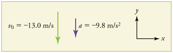
Since up is positive, the final position of the rock will be negative because it finishes below the starting point at [latex]{y}_{0}=0[/latex]. Similarly, the initial velocity is downward and therefore negative, as is the acceleration due to gravity. We expect the final velocity to be negative since the rock will continue to move downward.
Solution
- Identify the knowns. [latex]{y}_{0}=0[/latex];
[latex]{y}_{1}=-5\text{.}\text{10 m}[/latex];
[latex]{v}_{0}=-\text{13}\text{.0 m/s}[/latex];
[latex]a=-g=-9\text{.}\text{80 m}{\text{/s}}^{2}[/latex]. - Choose the kinematic equation that makes it easiest to solve the problem. The equation [latex]{v}^{2}={v}_{0}^{2}+2a\left(y-{y}_{0}\right)[/latex] works well because the only unknown in it is [latex]v[/latex]. (We will plug [latex]{y}_{1}[/latex] in for [latex]y[/latex].)
- Enter the known values
[latex]{v}^{2}={\left(-\text{13}\text{.}\text{0 m/s}\right)}^{2}+2\left(-9\text{.}{\text{80 m/s}}^{2}\right)\left(-5\text{.}\text{10 m}-\text{0 m}\right)=\text{268}\text{.}{\text{96 m}}^{2}{\text{/s}}^{2},[/latex]where we have retained extra significant figures because this is an intermediate result.
Taking the square root, and noting that a square root can be positive or negative, gives[latex]v=±\text{16}\text{.4 m/s}.[/latex]The negative root is chosen to indicate that the rock is still heading down. Thus,
[latex]v=-\text{16}\text{.4 m/s}.[/latex]
Discussion
Note that this is exactly the same velocity the rock had at this position when it was thrown straight upward with the same initial speed. (See Example 5.1 and Figure 5.5(a).) This is not a coincidental result. Because we only consider the acceleration due to gravity in this problem, the speed of a falling object depends only on its initial speed and its vertical position relative to the starting point. For example, if the velocity of the rock is calculated at a height of 8.10 m above the starting point when the initial velocity is 13.0 m/s straight up, a result of [latex]±3\text{.}\text{20 m/s}[/latex] is obtained. Here both signs are meaningful; the positive value occurs when the rock is at 8.10 m and heading up, and the negative value occurs when the rock is at 8.10 m and heading back down. It has the same speed but the opposite direction.
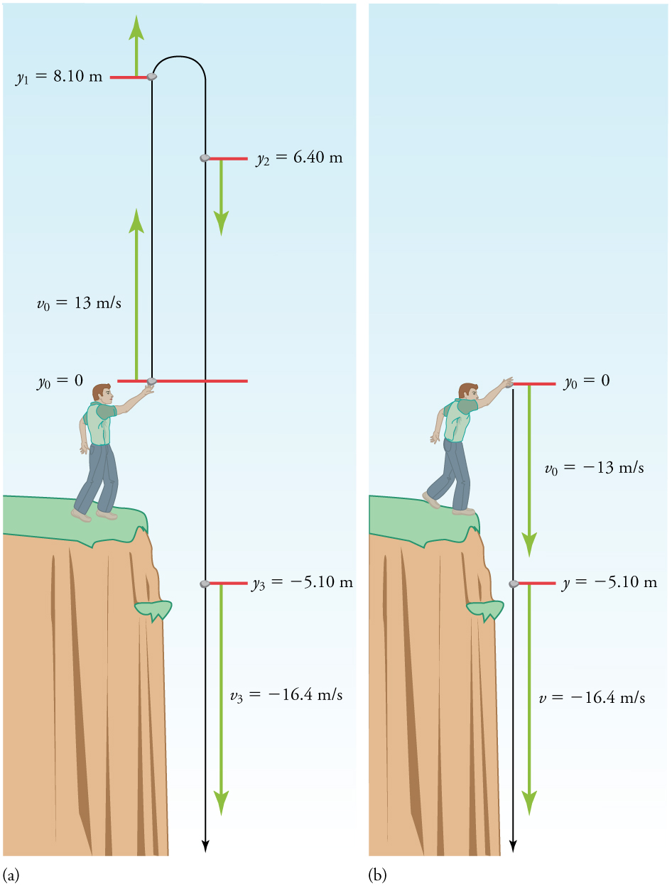
Another way to look at it is this: When the rock is thrown up with an initial velocity of [latex]\text{13}\text{.0 m/s}[/latex]. It rises and then falls back down. When its position is [latex]y=0[/latex] on its way back down, its velocity is [latex]-\text{13}\text{.0 m/s}[/latex]. That is, it has the same speed on its way down as on its way up. We would then expect its velocity at a position of [latex]y=-5\text{.}\text{10 m}[/latex] to be the same whether we have thrown it upwards at [latex]+\text{13}\text{.0 m/s}[/latex] or thrown it downwards at [latex]-\text{13}\text{.0 m/s}[/latex]. The velocity of the rock on its way down from [latex]y=0[/latex] is the same whether we have thrown it up or down to start with, as long as the speed with which it was initially thrown is the same.
Example 5.3: Find g from Data on a Falling Object
The acceleration due to gravity on Earth differs slightly from place to place, depending on topography (e.g., whether you are on a hill or in a valley) and subsurface geology (whether there is dense rock like iron ore as opposed to light rock like salt beneath you.) The precise acceleration due to gravity can be calculated from data taken in an introductory physics laboratory course. An object, usually a metal ball for which air resistance is negligible, is dropped and the time it takes to fall a known distance is measured. See, for example, Figure 5.6. Very precise results can be produced with this method if sufficient care is taken in measuring the distance fallen and the elapsed time.
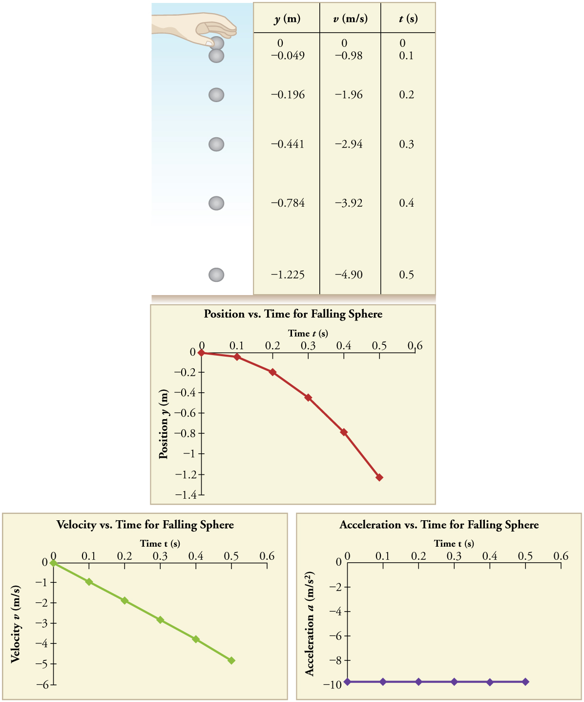
Suppose the ball falls 1.0000 m in 0.45173 s. Assuming the ball is not affected by air resistance, what is the precise acceleration due to gravity at this location?
Strategy
Draw a sketch.
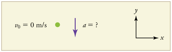
We need to solve for acceleration [latex]a[/latex]. Note that in this case, displacement is downward and therefore negative, as is acceleration.
Solution
- Identify the knowns. [latex]{y}_{0}=0[/latex];
[latex]y=–1\text{.0000 m}[/latex];
[latex]t=0\text{.45173}[/latex]; [latex]{v}_{0}=0[/latex]. - Choose the equation that allows you to solve for [latex]a[/latex] using the known values.
[latex]y={y}_{0}+{v}_{0}t+\frac{1}{2}{\text{at}}^{2}[/latex]
-
Substitute 0 for [latex]{v}_{0}[/latex] and rearrange the equation to solve for [latex]a[/latex]. Substituting 0 for [latex]{v}_{0}[/latex] yields[latex]y={y}_{0}+\frac{1}{2}{\text{at}}^{2}\text{.}[/latex]
Solving for [latex]a[/latex] gives
[latex]a=\frac{2\left(y-{y}_{0}\right)}{{t}^{2}}\text{.}[/latex] - Substitute known values yields
[latex]a=\frac{2\left(-1\text{.}\text{0000 m – 0}\right)}{\left(0\text{.}\text{45173 s}\right)}^{2}=-9\text{.}{\text{8010 m/s}}^{2},[/latex]
so, because [latex]a=-g[/latex] with the directions we have chosen,
[latex]g=9\text{.}{\text{8010 m/s}}^{2}.[/latex]
Discussion
The negative value for [latex]a[/latex] indicates that the gravitational acceleration is downward, as expected. We expect the value to be somewhere around the average value of [latex]9\text{.}{\text{80 m/s}}^{2}[/latex], so [latex]9\text{.}{\text{8010 m/s}}^{2}[/latex] makes sense. Since the data going into the calculation are relatively precise, this value for [latex]g[/latex] is more precise than the average value of [latex]9\text{.}{\text{80 m/s}}^{2}[/latex]; it represents the local value for the acceleration due to gravity.
Check Your Understanding
A chunk of ice breaks off a glacier and falls [latex]30.0\ \text{m}[/latex] before it hits the water. Assuming it falls freely (that is, with no air resistance), how long does it take to hit the water?
We are given:
-
Initial position: [latex]y_0 = 0[/latex]
-
Final position: [latex]y = -30.0\ \text{m}[/latex]
-
Initial velocity: [latex]v_0 = 0[/latex] (the object is dropped)
-
Acceleration: [latex]a = -g = -9.80\ \text{m/s}^2[/latex]
We use the following kinematic equation:
[latex]y = y_0 + v_0 t + \frac{1}{2} a t^2[/latex]
Substitute known values:
[latex]-30.0 = 0 + 0 - \frac{1}{2}(9.80)t^2[/latex]
Solve for [latex]t[/latex]:
[latex]t^2 = \frac{2(-30.0)}{-9.80} = \frac{-60.0}{-9.80} = 6.12[/latex]
[latex]t = \sqrt{6.12} \approx 2.47\ \text{s}[/latex]
Answer: It takes approximately [latex]2.5\ \text{s}[/latex] for the piece of ice to hit the water.
PhET Explorations: Equation Grapher
Explore how different polynomial terms contribute to the shape of a graph. With the Equation Grapher simulation, you can:
-
Graph equations like [latex]y = bx[/latex], [latex]y = ax^2[/latex], and more.
-
Adjust constants to see how they affect the curve.
-
Combine terms to visualize full polynomial functions.
Gravity in Everyday Life and Astronomy
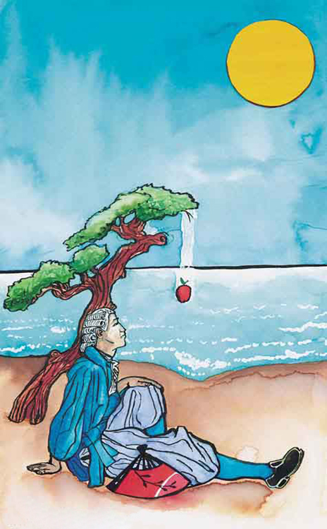
From aching feet to falling apples to orbiting moons, all these phenomena are governed by gravity—the attractive force between all masses. This force holds planets in orbit, forms galaxies, and even affects biological functions like posture and blood circulation.
Sir Isaac Newton was the first to formulate a universal law that explained both terrestrial and celestial motion using a single principle. The legend of the falling apple (Figure 5.8) symbolizes his insight: if gravity acts on an apple, could it not also reach the Moon—and beyond?
Newton’s Law of Universal Gravitation
Newton’s universal law of gravitation states:
Every particle in the universe attracts every other particle with a force that is proportional to the product of their masses and inversely proportional to the square of the distance between their centers.
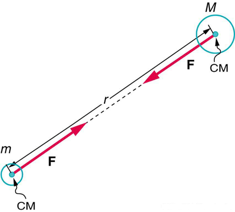
Mathematically, the gravitational force [latex]F[/latex] between two objects of mass [latex]m[/latex] and [latex]M[/latex], separated by a distance [latex]r[/latex], is:
[latex]F = G \frac{mM}{r^2}[/latex]
-
[latex]F[/latex]: gravitational force in newtons (N)
-
[latex]G[/latex]: gravitational constant,
[latex]G = 6.674 \times 10^{-11} , \frac{\text{N} \cdot \text{m}^2}{\text{kg}^2}[/latex] -
[latex]m, M[/latex]: masses in kilograms (kg)
-
[latex]r[/latex]: distance between centers of mass in meters (m)
This relationship is illustrated in Figure 5.9, where the gravitational force acts along the line connecting the centers of mass of the two bodies. Consistent with Newton’s third law, both bodies experience forces of equal magnitude in opposite directions.
Center of Mass and Simplification
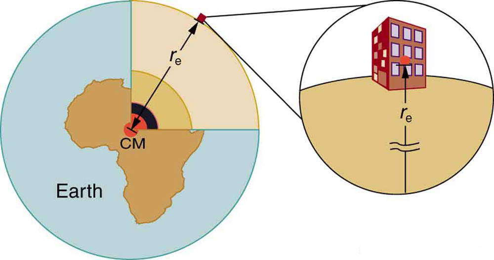
For extended bodies like planets or humans, we assume their mass is concentrated at a point—their center of mass. This simplifies gravitational calculations, particularly when the distance between objects is much larger than their size.
Deriving the Acceleration Due to Gravity [latex]g[/latex]
Let’s connect Newton’s law of gravitation to the acceleration of falling objects on Earth. Recall that weight is defined as:
[latex]F = mg[/latex]
Substituting into Newton’s gravitational equation:
[latex]mg = G \frac{mM}{r^2}[/latex]
Solving for [latex]g[/latex]:
[latex]g = G \frac{M}{r^2}[/latex]
Using Earth’s values:
-
[latex]M = 5.98 \times 10^{24} , \text{kg}[/latex]
-
[latex]r = 6.38 \times 10^6 , \text{m}[/latex] (Earth’s radius)
[latex]g = \left(6.67 \times 10^{-11} , \frac{\text{N} \cdot \text{m}^2}{\text{kg}^2} \right) \frac{5.98 \times 10^{24} , \text{kg}}{(6.38 \times 10^6 , \text{m})^2} = 9.80 , \text{m/s}^2[/latex]
This result is consistent with the observed acceleration due to gravity on Earth, and it shows that all objects—regardless of mass—fall at the same rate near Earth’s surface.
Figure 5.10 shows the gravitational interaction between Earth and an object, emphasizing that [latex]r[/latex] is the distance to Earth’s center.
Misconception Alert: Equal Force on Unequal Masses
One common misunderstanding is that heavier objects exert more gravitational force. While heavier objects do exert larger forces on lighter ones, Newton’s third law ensures the forces are equal and opposite. The difference lies in the acceleration, which is smaller for the more massive body.
Take-Home Experiment
Try dropping a marble, a spoon, and a ball from the same height. Do they hit the ground at the same time? Likely, yes. Now try a sheet of paper—its slower fall is due to air resistance, not gravitational mass.
Broader Context: Gravitational Force in Modern Physics
Although Newton’s law remains powerful, modern physics—especially Einstein’s General Relativity—treats gravity as the curvature of space-time rather than a force. Still, Newton’s equation accurately predicts planetary motion and everyday gravitational effects.
Preview of the Cavendish Experiment
In the next section, we’ll explore Henry Cavendish’s experiment, which provided the first accurate measurement of the gravitational constant [latex]G[/latex], enabling scientists to weigh Earth and validate Newton’s equation with laboratory-scale data.
Example 5.4: Earth’s Gravitational Force Is the Centripetal Force Making the Moon Move in a Curved Path
- Find the acceleration due to Earth’s gravity at the distance of the Moon.
- Calculate the centripetal acceleration needed to keep the Moon in its orbit (assuming a circular orbit about a fixed Earth), and compare it with the value of the acceleration due to Earth’s gravity that you have just found.
Strategy for (a)
This calculation is the same as the one finding the acceleration due to gravity at Earth’s surface, except that [latex]r[/latex]is the distance from the center of Earth to the center of the Moon. The radius of the Moon’s nearly circular orbit is [latex]3\text{.}\text{84}×{\text{10}}^{8}\phantom{\rule{0.25em}{0ex}}\text{m}[/latex].
Solution for (a)
Substituting known values into the expression for [latex]g[/latex] found above, remembering that [latex]M[/latex] is the mass of Earth not the Moon, yields
Strategy for (b)
Centripetal acceleration can be calculated using either form of
We choose to use the second form:
where [latex]\omega[/latex] is the angular velocity of the Moon about Earth.
Solution for (b)
Given that the period (the time it takes to make one complete rotation) of the Moon’s orbit is 27.3 days, (d) and using
we see that
The centripetal acceleration is
The direction of the acceleration is toward the center of the Earth.
Discussion
The centripetal acceleration of the Moon found in (b) differs by less than 1% from the acceleration due to Earth’s gravity found in (a). This agreement is approximate because the Moon’s orbit is slightly elliptical, and Earth is not stationary (rather the Earth-Moon system rotates about its center of mass, which is located some 1700 km below Earth’s surface). The clear implication is that Earth’s gravitational force causes the Moon to orbit Earth.
Earth and Moon: Mutual Gravitation
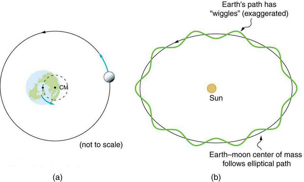
Although it seems the Moon orbits a stationary Earth, this is not entirely true. According to Newton’s third law, the gravitational force the Earth exerts on the Moon is matched by an equal and opposite force the Moon exerts on Earth.
Both Earth and the Moon orbit their common center of mass, which lies inside Earth but not at its exact center (Figure 5.11). This mutual orbit causes small “wiggles” in Earth’s path around the Sun—subtle variations observable in the motion of stars that reveal the presence of exoplanets orbiting them.
Tides: Evidence of the Moon’s Gravitational Pull
One of the most visible consequences of the Moon’s gravity is tides on Earth’s oceans. Because water is mobile, the Moon’s gravity pulls more strongly on the side of Earth closest to it, creating a high tide. A second high tide occurs on the far side, where Earth is pulled away from the water (Figure 5.12).
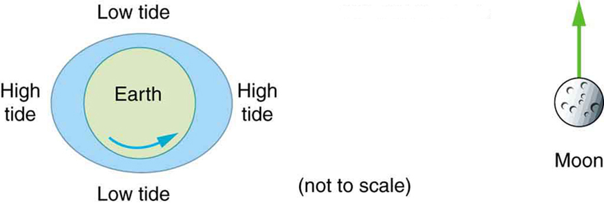
As Earth rotates under these tidal bulges, most coastal locations experience two high tides and two low tides every 24 hours and 50.4 minutes, aligning with the Moon’s orbital motion.
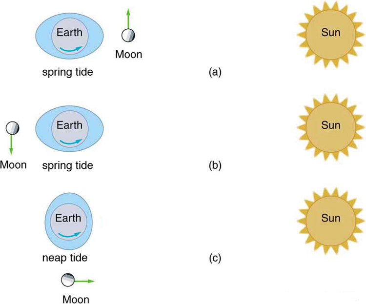
The Sun also contributes to tides, but its influence is only about half that of the Moon. When the Sun, Earth, and Moon align (new or full moon), their gravitational effects reinforce one another, creating spring tides, the highest tides. When they form a right angle (first or third quarter), the effects partially cancel, causing neap tides, the smallest tides (Figure 5.13).
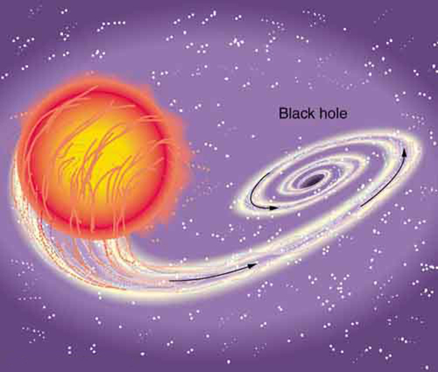
Tidal effects also occur in extreme conditions—near black holes, for instance. These objects generate such intense tidal forces that they can tear matter from nearby stars, forming luminous accretion disks (Figure 5.14).
“Weightlessness” and Microgravity in Orbit
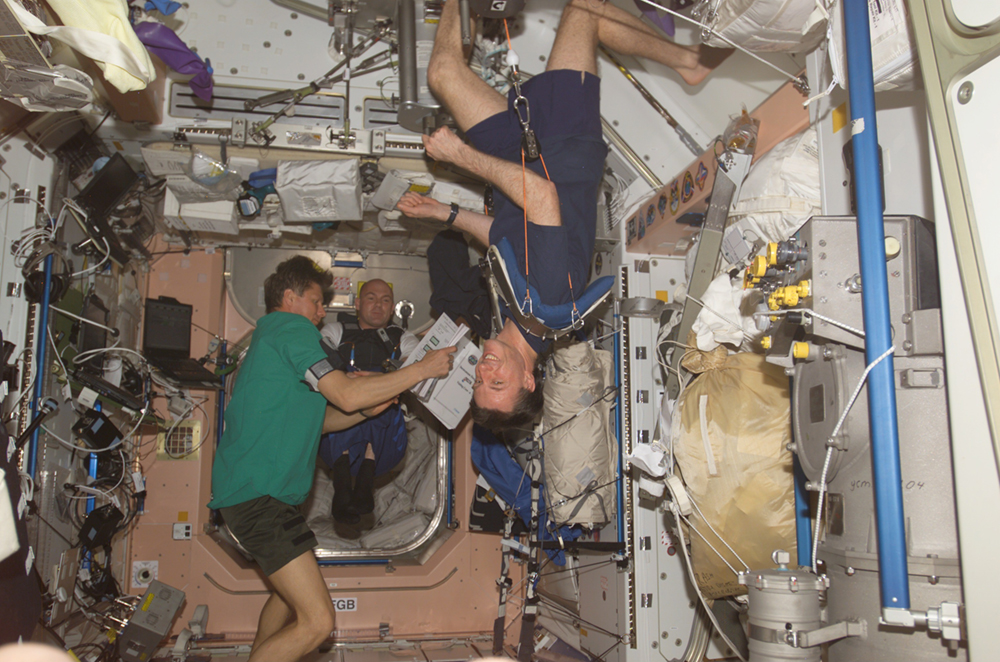
Astronauts in orbit appear weightless, but gravity is still acting on them. They are in free fall, continuously falling toward Earth but traveling forward fast enough to remain in orbit. This state is known as apparent weightlessness, illustrated by astronauts aboard the International Space Station (Figure 5.15).
In such environments, microgravity—very small net acceleration—is experienced. This has significant biological and technological implications:
-
Muscle atrophy and bone density loss are common in astronauts.
-
Cardiovascular adaptations occur due to loss of pressure gradients.
-
The immune system weakens, increasing infection risk.
-
Some bacteria grow faster in space, while others produce more antibiotics.
-
High-quality crystal growth in microgravity enables advanced materials research.
Plants, which rely on gravity to orient their roots and shoots, may play vital roles in life support systems during long-term space missions. However, more research is needed on how microgravity affects their development.
The Cavendish Experiment: Measuring [latex]G[/latex]
The gravitational constant [latex]G[/latex] was first measured by Henry Cavendish in 1798 using a torsion balance apparatus (Figure 5.16). This device measured the tiny attraction between lead spheres, allowing Cavendish to calculate the strength of gravity between known masses.
Using Newton’s law:
[latex]F = G \frac{mM}{r^2}[/latex]
and substituting [latex]F = mg[/latex] (the object’s weight), we get:
[latex]mg = G \frac{mM}{r^2}[/latex]
Canceling [latex]m[/latex]:
[latex]g = G \frac{M}{r^2}[/latex]
Solving for Earth’s mass:
[latex]M = \frac{gr^2}{G}[/latex]
With accurate values for [latex]g[/latex], [latex]r[/latex] (Earth’s radius), and [latex]G[/latex], we can compute Earth’s mass. This was one of the first scientific estimates of a planet’s mass.

Modern Advances in Gravitational Experiments
Experiments following Cavendish’s method have refined our understanding of gravity:
-
Eötvös-type experiments confirmed that gravity acts equally on all substances, supporting the equivalence principle.
-
Modern torsion balances test gravity’s behavior at millimeter scales, searching for deviations from the inverse-square law.
-
These tests also probe for a fifth force or signs of quantum gravity.
-
Recent studies confirm that gravitational energy contributes to mass, in line with general relativity.
These continued efforts help us verify and extend Newton’s ideas, bridging toward modern theories of gravity.
Gravitational Orbits: A Universal Phenomenon
From the Moon’s orbit around Earth to artificial satellites and distant star systems, gravitationally bound orbits are everywhere. These orbits include:
-
Earth’s natural and artificial satellites
-
Planetary orbits around the Sun
-
Binary star systems
-
Galaxy clusters held together by mutual gravitational attraction
Although real-world gravitational systems can be complex and require numerical computation, many important insights come from examining simplified orbital models governed purely by Newtonian gravity.
Simplifying Assumptions for Orbital Motion
To explore orbital motion analytically, we consider a special but very common case:
-
A small mass [latex]m[/latex] (e.g., a satellite or planet) orbits a much larger mass [latex]M[/latex] (e.g., a planet or star).
-
The gravitational interaction dominates, and outside influences from other bodies are negligible.
-
The center of mass lies within [latex]M[/latex], allowing us to approximate it as stationary.
This idealization applies to:
-
The Moon orbiting Earth
-
Earth and other planets orbiting the Sun
-
Moons of Jupiter, Saturn, and other planets
-
Artificial satellites orbiting Earth
These assumptions provide the foundation for understanding Kepler’s laws of planetary motion.
Kepler’s Laws of Planetary Motion
Developed by Johannes Kepler in the early 1600s, these laws describe planetary orbits based on the extensive astronomical data collected by Tycho Brahe. Though originally formulated to describe planets orbiting the Sun, Kepler’s laws apply to any object in gravitational orbit under the conditions noted above.
Kepler’s First Law: Elliptical Orbits
The orbit of each planet is an ellipse, with the Sun at one focus.
An ellipse is a closed, elongated curve defined by two fixed points called foci. The sum of the distances from any point on the ellipse to each focus is constant (Figure 5.17a). A circle is a special case of an ellipse in which both foci coincide.
For any gravitationally bound object orbiting another, the path is elliptical, with the more massive body (e.g., the Sun or a planet) located at one focus (Figure 5.17b).
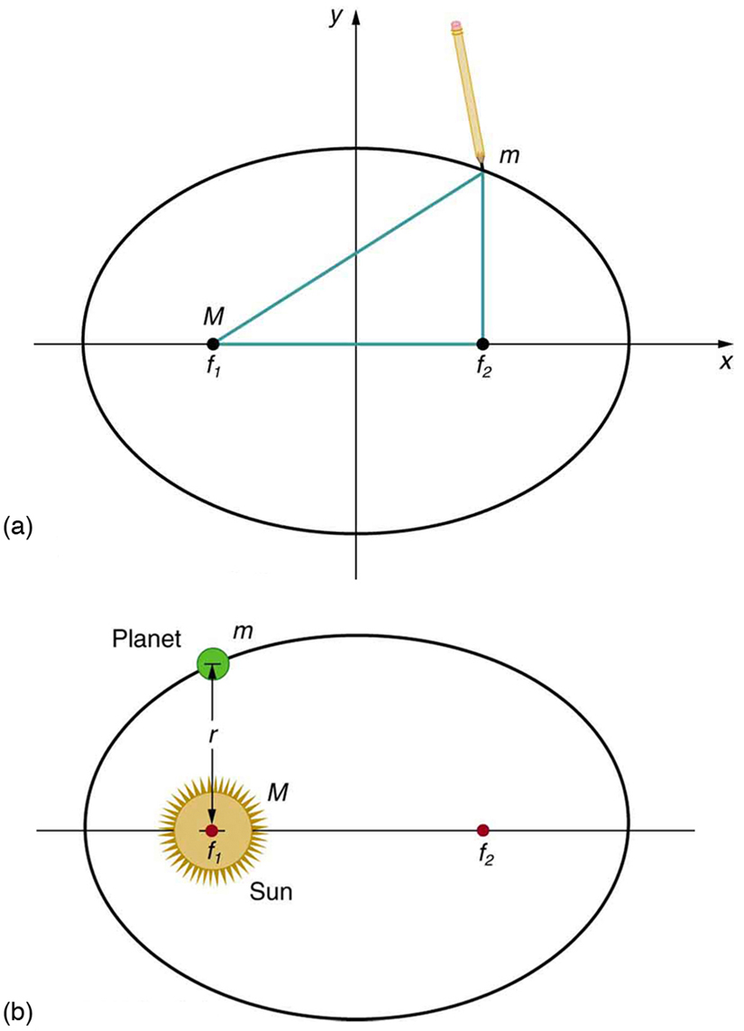
(b) In a gravitational orbit, the smaller body [latex]m[/latex] moves around the larger mass [latex]M[/latex] along an elliptical path with [latex]M[/latex] at one focus.
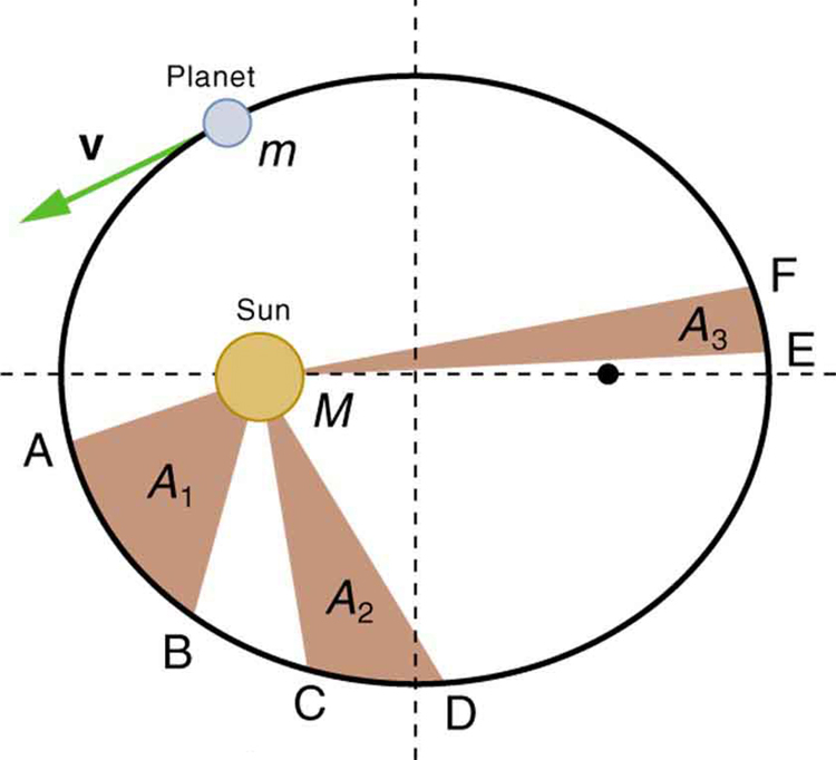
Kepler’s Second Law: Equal Areas in Equal Times
A line drawn from the orbiting object to the central body sweeps out equal areas in equal intervals of time.
This law implies that the object moves faster when it is closer to the central mass and slower when it is farther away (Figure 5.18). The varying speed maintains the constant areal rate of motion, a consequence of conservation of angular momentum.
Kepler’s Third Law: Harmonic Law
The square of the orbital period of a planet is proportional to the cube of the average orbital radius.
Mathematically:
[latex]\frac{T_1^2}{T_2^2} = \frac{r_1^3}{r_2^3}[/latex]
Here:
-
[latex]T_1[/latex] and [latex]T_2[/latex] are the orbital periods of two planets, and
-
[latex]r_1[/latex] and [latex]r_2[/latex] are their respective average orbital radii.
This relation applies only when both small masses orbit the same large central mass. The law is empirical—it describes the motion but does not explain the underlying cause. The physical origin (gravitational force) was later provided by Newton.
💡 Note: While Kepler formulated his laws for planets orbiting the Sun, these laws apply more generally to any gravitational two-body system where a small mass orbits a much larger one.
Example 5.5: Find the Time for One Orbit of an Earth Satellite
Given that the Moon orbits Earth each 27.3 d and that it is an average distance of [latex]3.84×{\text{10}}^{8}\phantom{\rule{0.25em}{0ex}}\text{m}[/latex] from the center of Earth, calculate the period of an artificial satellite orbiting at an average altitude of 1500 km above Earth’s surface.
Strategy
The period, or time for one orbit, is related to the radius of the orbit by Kepler’s third law, given in mathematical form in [latex]\frac{{T}_{1}^{ 2}}{{T}_{2}^{ 2}}=\frac{{r}_{1}^{ 3}}{{r}_{2}^{ 3}}[/latex]. Let us use the subscript 1 for the Moon and the subscript 2 for the satellite. We are asked to find [latex]{T}_{2}[/latex]. The given information tells us that the orbital radius of the Moon is [latex]{r}_{1}=3\text{.}\text{84}×{\text{10}}^{8}\phantom{\rule{0.25em}{0ex}}\text{m}[/latex], and that the period of the Moon is [latex]{T}_{1}=\text{27.3 d}[/latex]. The height of the artificial satellite above Earth’s surface is given, and so we must add the radius of Earth (6380 km) to get [latex]{r}_{2}=\left(\text{1500}+\text{6380}\right)\phantom{\rule{0.25em}{0ex}}\text{km}=\text{7880}\phantom{\rule{0.25em}{0ex}}\text{km}[/latex]. Now all quantities are known, and so [latex]{T}_{2}[/latex] can be found.
Solution
Kepler’s third law is
To solve for [latex]{T}_{2}[/latex], we cross-multiply and take the square root, yielding
Substituting known values yields
Discussion
This is a reasonable period for a satellite in a fairly low orbit. It is interesting that any satellite at this altitude will orbit in the same amount of time. This fact is related to the condition that the satellite’s mass is small compared with that of Earth.
Newton’s Laws Lead to Kepler’s Third Law
Let us derive Kepler’s third law using Newton’s law of gravitation and Newton’s second law. Consider a satellite of mass [latex]m[/latex] orbiting a much larger central mass [latex]M[/latex] (e.g., a planet orbiting the Sun). We assume a circular orbit for simplicity. Gravity provides the centripetal force that keeps the satellite in orbit:
[latex]F_{\text{net}} = ma_{\text{c}} = m \frac{v^2}{r}[/latex]
Now, applying Newton’s law of universal gravitation as the source of this centripetal force:
[latex]F_{\text{gravity}} = G \frac{mM}{r^2}[/latex]
Equating the two forces:
[latex]G \frac{mM}{r^2} = m \frac{v^2}{r}[/latex]
Canceling [latex]m[/latex] from both sides and solving for [latex]v^2[/latex]:
[latex]G \frac{M}{r} = v^2[/latex]
Since the orbital speed [latex]v[/latex] is related to the period [latex]T[/latex] of revolution by the circumference of the orbit:
[latex]v = \frac{2\pi r}{T}[/latex]
Substitute this into the expression for [latex]v^2[/latex]:
[latex]G \frac{M}{r} = \left(\frac{2\pi r}{T}\right)^2 = \frac{4\pi^2 r^2}{T^2}[/latex]
Solving for [latex]T^2[/latex]:
[latex]T^2 = \frac{4\pi^2}{GM} r^3[/latex]
This shows that for any object orbiting the same central mass [latex]M[/latex], the square of the orbital period is proportional to the cube of the orbital radius:
[latex]\frac{T_1^2}{T_2^2} = \frac{r_1^3}{r_2^3}[/latex]
This is Kepler’s third law. It applies to all satellites orbiting the same parent body.
Using Kepler’s Third Law to Determine Mass
Rewriting the result:
[latex]\frac{r^3}{T^2} = \frac{GM}{4\pi^2}[/latex]
This formula allows us to determine the mass [latex]M[/latex] of the central body if we know the satellite’s orbital radius and period. This method has been extensively used to calculate the masses of stars, planets, and galaxies.
Table of Orbital Data and [latex]r^3 / T^2[/latex] Ratios
The table below shows orbital data for various bodies orbiting the Sun and Jupiter. The values of [latex]r^3 / T^2[/latex] remain constant (to within measurement uncertainty), confirming the predictive power of Kepler’s third law and Newtonian gravity.
Small deviations arise due to:
-
Uncertainties in measurement
-
Gravitational perturbations by other bodies
Such perturbations have even led to the discovery of new planets and moons, a triumph of Newtonian gravity.
Simplicity and the Power of Universal Laws
Kepler’s laws describe planetary motion, but Newton’s gravitational theory explains them. This marked a shift in science—from description to causation through universal laws.
“Truth is ever to be found in simplicity.” — Isaac Newton
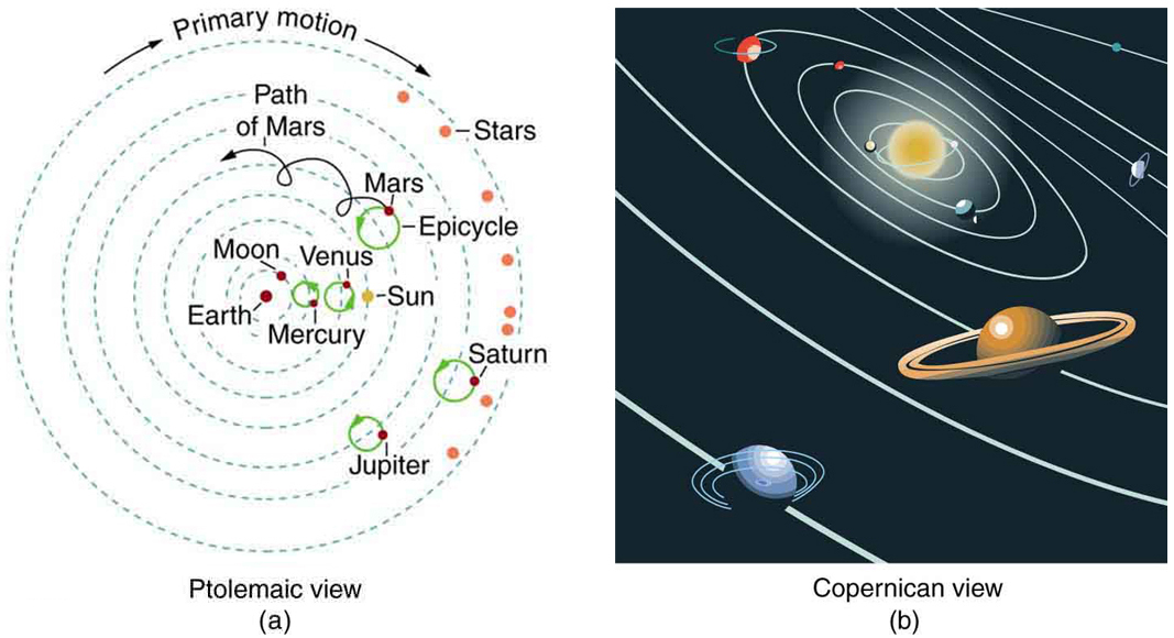
The Copernican model (Figure 5.19(b)) exemplifies this simplicity, explaining planetary motion using a few core principles. By contrast, the Ptolemaic model (Figure 5.19(a)) relied on complex geometrical constructions without causal explanation.
Section Summary
-
An object in free fall experiences constant acceleration if air resistance is negligible.
-
On Earth, all free-falling objects accelerate downward due to gravity, with acceleration [latex]g[/latex] averaging
[latex]g = 9.80\ \text{m/s}^2.[/latex]
-
The sign of the acceleration [latex]a[/latex] depends on the choice of coordinate system:
-
If upward is chosen as positive, then
[latex]a = -g = -9.80\ \text{m/s}^2[/latex] (acceleration is negative)
-
If downward is chosen as positive, then
[latex]a = +g = 9.80\ \text{m/s}^2[/latex] (acceleration is positive)
-
-
Since acceleration is constant, the kinematic equations can be applied by substituting either [latex]+g[/latex] or [latex]-g[/latex] for [latex]a[/latex] as appropriate.
-
For free-falling objects, up is normally taken as positive for displacement, velocity, and acceleration.
-
Newton’s Universal Law of Gravitation states that:
Every mass attracts every other mass through a force proportional to the product of their masses and inversely proportional to the square of the distance between them.
Mathematically:
[latex]F = G \frac{mM}{r^2}[/latex]
-
[latex]F[/latex] is the gravitational force,
-
[latex]G = 6.674 \times 10^{-11} , \text{N} \cdot \text{m}^2/\text{kg}^2[/latex],
-
[latex]m[/latex] and [latex]M[/latex] are the masses involved,
-
[latex]r[/latex] is the distance between their centers of mass.
This law applies universally—from falling apples to orbiting galaxies—and continues to be confirmed by experiments and observations.
-
-
Kepler’s third law states that [latex]T^2 \propto r^3[/latex] for orbiting bodies.
-
It can be derived from Newton’s second law and his law of gravitation.
-
The resulting formula [latex]T^2 = \frac{4\pi^2}{GM} r^3[/latex] connects orbit period to central mass and radius.
-
These ideas highlight the unity and simplicity of physics, showing how one fundamental force explains a wide variety of natural phenomena.
Glossary
- free-fall
- the state of movement that results from gravitational force only
- acceleration due to gravity
- acceleration of an object as a result of gravity
